FIRST Robotics Competition Control System
Welcome to the FIRST® Robotics Competition Control System Documentation! This site contains everything you need to know for programming a competition robot!
Community translations can be found in a variety of languages in the bottom-left menu.
Returning Teams
If you are a returning team, please check out the overview of changes from 2021 to 2022 and the cards below for a refresher.
New Teams
The Zero-to-Robot tutorial will guide you through preparation, wiring and programming a basic robot!
Hardware Overview
An overview of the hardware components available to teams.
Software Overview
An overview of the software components and tools available to teams.
Programming Basics
Documentation that is useful throughout a team’s programming process.
Advanced Programming
Documentation that is suited toward veteran teams. This includes content such as Path Planning and Kinematics.
Hardware
Hardware tutorials and content available for teams.
Romi Robot
The Romi Robot is a low-cost Raspberry Pi based platform for practicing WPILib programming.
API Documentation
Java and C++ class documentation.
Software Tools
Essential tooling such as FRC Driver Station, Dashboards, roboRIO Imaging Tool and more.
Example Projects
This section showcases the available example projects that teams can reference in VS Code.
Status Light Quick Reference
Quick reference guide for the status lights on a variety of FRC hardware.
3rd Party Libraries
Tutorial on adding 3rd party libraries such as CTRE and REV to your robot project.
Introduction
Welcome to the official documentation home for the FIRST® Robotics Competition Control System and WPILib software packages. This page is the primary resource documenting the use of the FRC® Control System (including wiring, configuration and software) as well as the WPILib libraries and tools.
New to Programming?
These pages cover the specifics of the WPILib libraries and the FRC Control System and do not describe the basics of using the supported programming languages. If you would like resources on learning the supported programming languages check out the recommendations below:
Note
You can continue with this Zero-to-Robot section to get a functioning basic robot without knowledge of the programming language. To go beyond that, you will need to be familiar with the language you choose to program in.
Java
Head First Java 2nd Edition is a very beginner friendly introduction to programming in Java (ISBN-10: 0596009208).
C++
Programming: Principles and Practice Using C++ 2nd Edition is an introduction to C++ by the creator of the language himself (ISBN-10: 0321992784).
C++ Primer Plus 6th Edition (ISBN-10: 0321776402).
LabVIEW
Zero to Robot
The remaining pages in this tutorial are designed to be completed in order to go from zero to a working basic robot. The documents will walk you through wiring your robot, installation of all needed software, configuration of hardware, and loading a basic example program that should allow your robot to operate. When you complete a page, simply click Next to navigate to the next page and continue with the process. When you’re done, you can click Next to continue to an overview of WPILib in C++/Java or jump back to the home page using the logo at the top left to explore the rest of the content.
Step 1: Building your Robot
An overview of the available control system hardware can be found here.
How to Wire an FRC Robot
Note
This document details the wiring of a basic electronics board for bench-top testing.
Some images shown in this section reflect the setup for a Robot Control System using Victor SPX Motor Controllers. Wiring diagram and layout should be similar for other motor controllers. Where appropriate, two sets of images are provided to show connections using controllers with and without integrated wires.
Gather Materials
Locate the following control system components and tools
Kit Materials:
Power Distribution Panel (PDP)
roboRIO
Pneumatics Control Module (PCM)
Voltage Regulator Module (VRM)
OpenMesh radio (with power cable and Ethernet cable)
Robot Signal Light (RSL)
4x SPARK MAX or other motor controllers
2x PWM y-cables
120A Circuit breaker
4x 40A Circuit breaker
6 AWG (16 \(mm^2\)) Red wire
10 AWG (6 \(mm^2\)) Red/Black wire
18 AWG (1 \(mm^2\)) Red/Black wire
22 AWG (0.5 \(mm^2\)) Yellow/Green twisted CAN cable
16x 10-12 AWG (4 - 6 \(mm^2\)) (Yellow) ring terminals (8x quick disconnect pairs if using integrated wire controllers)
2x Anderson SB50 battery connectors
6 AWG (16 \(mm^2\)) Terminal lugs
12V Battery
Red/Black Electrical tape
Dual Lock material or fasteners
Zip ties
1/4” or 1/2” (6-12 mm) plywood
Tools Required:
Wago Tool or small flat-head screwdriver
Very small flat head screwdriver (eyeglass repair size)
Philips head screw driver
5 mm Hex key (3/16” may work if metric is unavailable)
1/16” Hex key
Wire cutters, strippers, and crimpers
7/16” (11 mm may work if imperial is unavailable) box end wrench or nut driver
Create the Base for the Control System
For a benchtop test board, cut piece of 1/4” or 1/2” (6-12 mm) material (wood or plastic) approximately 24” x 16” (60 x 40 cm). For a Robot Quick Build control board see the supporting documentation for the proper size board for the chosen chassis configuration.
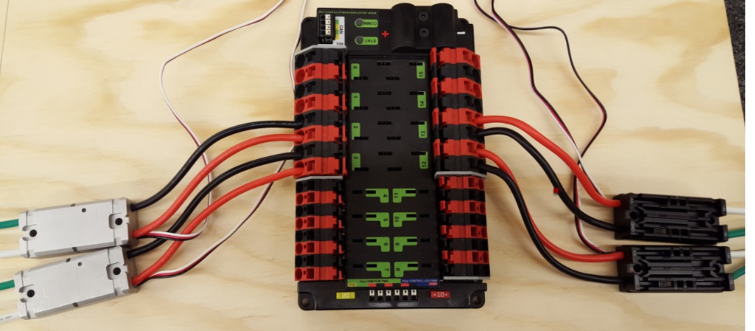
Layout the Core Control System Components
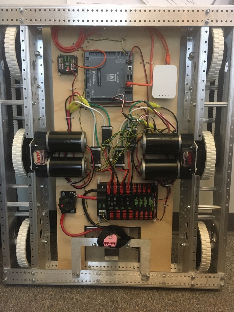
Lay out the components on the board. An example layout is shown in the image above.
Fasten Components
Using the Dual Lock or hardware, fasten all components to the board. Note that in many FRC games robot-to-robot contact may be substantial and Dual Lock alone is unlikely to stand up as a fastener for many electronic components. Teams may wish to use nut and bolt fasteners or (as shown in the image above) cable ties, with or without Dual Lock to secure devices to the board.
Attach Battery Connector to PDP
Requires: Battery Connector, 6 AWG (16 \(mm^2\)) terminal lugs, 1/16” Allen, 5 mm Allen, 7/16” (11 mm) Box end
Attach terminal lugs to battery connector:
Using a 1/16” Allen wrench, remove the two screws securing the PDP terminal cover.
Using a 5 mm Allen wrench (3/16”), remove the negative (-) bolt and washer from the PDP and fasten the negative terminal of the battery connector.
Using a 7/16” (11 mm) box end wrench, remove the nut on the “Batt” side of the main breaker and secure the positive terminal of the battery connector
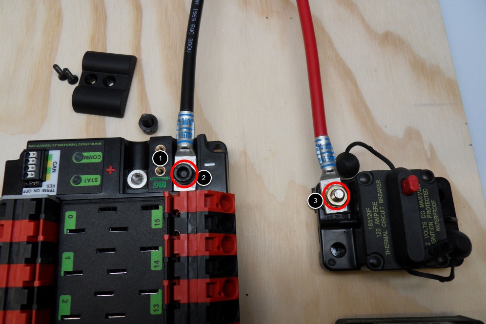
Wire Breaker to PDP
Requires: 6 AWG (16 \(mm^2\)) red wire, 2x 6 AWG (16 \(mm^2\)) terminal lugs, 5 mm Allen, 7/16” (11 mm) box end
Secure one terminal lug to the end of the 6 AWG (16 \(mm^2\)) red wire. Using the 7/16” (11 mm) box end, remove the nut from the “AUX” side of the 120A main breaker and place the terminal over the stud. Loosely secure the nut (you may wish to remove it shortly to cut, strip, and crimp the other end of the wire). Measure out the length of wire required to reach the positive terminal of the PDP.
Cut, strip, and crimp the terminal to the 2nd end of the red 6 AWG (16 \(mm^2\)) wire.
Using the 7/16” (11 mm) box end, secure the wire to the “AUX” side of the 120A main breaker.
Using the 5 mm Allen wrench, secure the other end to the PDP positive terminal.
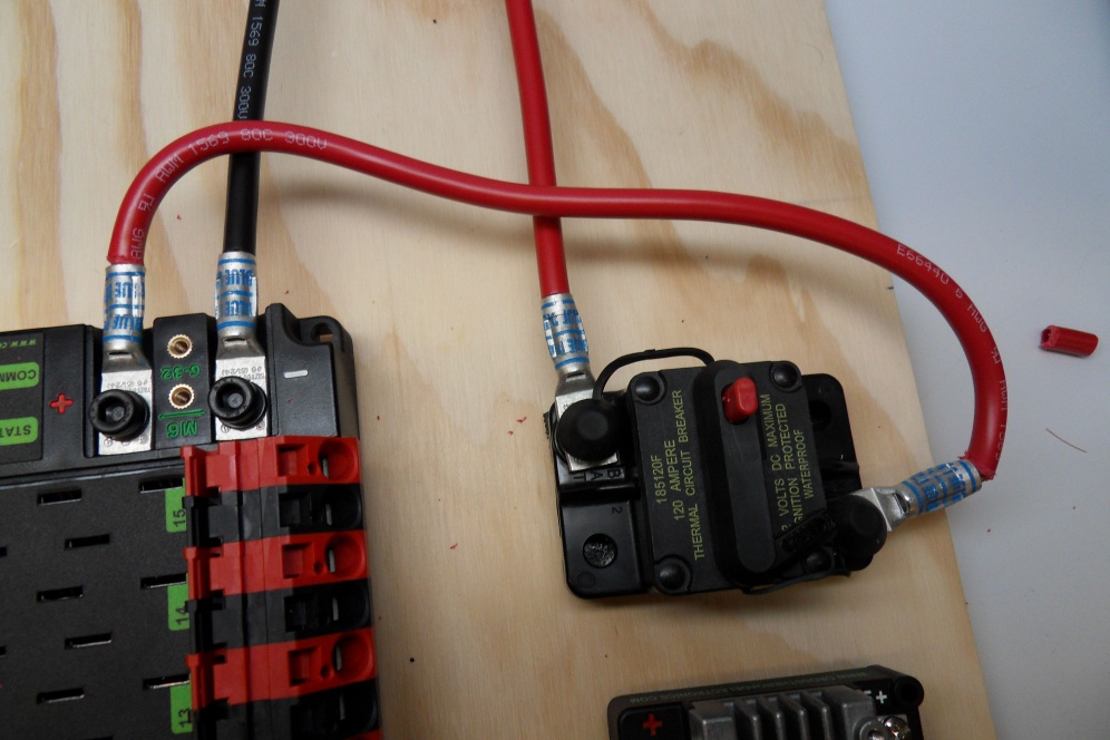
Insulate PDP connections
Requires: 1/16” Allen, Electrical tape
Using electrical tape, insulate the two connections to the 120A breaker. Also insulate any part of the PDP terminals which will be exposed when the cover is replaced. One method for insulating the main breaker connections is to wrap the stud and nut first, then use the tape wrapped around the terminal and wire to secure the tape.
Using the 1/16” Allen wrench, replace the PDP terminal cover
Wago connectors
The next step will involve using the Wago connectors on the PDP. To use the Wago connectors, insert a small flat blade screwdriver into the rectangular hole at a shallow angle then angle the screwdriver upwards as you continue to press in to actuate the lever, opening the terminal. Two sizes of Wago connector are found on the PDP:
Small Wago connector: Accepts 10 - 24 AWG (0.25 - 6 \(mm^2\)), strip 11-12 mm (~7/16”)
Large Wago connector: Accepts 6 - 12 AWG (4 - 16 \(mm^2\)), strip 12-13 mm (~1/2”)
To maximize pullout force and minimize connection resistance wires should not be tinned (and ideally not twisted) before inserting into the Wago connector.
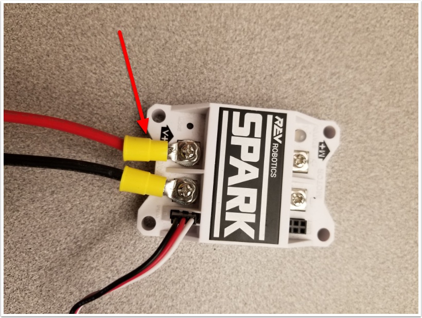
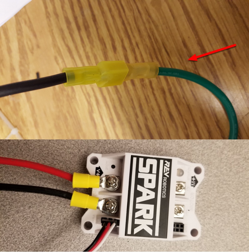
Motor Controller Power
Requires: Wire Stripper, Small Flat Screwdriver, 10 or 12 AWG (4 - 6 \(mm^2\)) wire, 10 or 12 AWG (4 - 6 \(mm^2\)) fork/ring terminals (terminal controllers only), wire crimper
For SPARK MAX or other wire integrated motor controllers (top image):
Cut and strip the red and black power input wires, then insert into one of the 40A (larger) Wago terminal pairs.
For terminal motor controllers (bottom image):
Cut red and black wire to appropriate length to reach from one of the 40A (larger) Wago terminal pairs to the input side of the motor controller (with a little extra for the length that will be inserted into the terminals on each end)
Strip one end of each of the wires, then insert into the Wago terminals.
Strip the other end of each wire, and crimp on a ring or fork terminal
Attach the terminal to the motor controller input terminals (red to +, black to -)
Weidmuller Connectors
Warning
The correct strip length is ~5/16” (~8 mm), not the 5/8” (~16 mm) mentioned in the video.
A number of the CAN and power connectors in the system use a Weidmuller LSF series wire-to-board connector. There are a few things to keep in mind when using this connector for best results:
Wire should be 16 AWG (1.5 \(mm^2\)) to 24 AWG (0.25 \(mm^2\)) (consult rules to verify required gauge for power wiring)
Wire ends should be stripped approximately 5/16 (~8 mm)”
To insert or remove the wire, press down on the corresponding “button” to open the terminal
After making the connection check to be sure that it is clean and secure:
Verify that there are no “whiskers” outside the connector that may cause a short circuit
Tug on the wire to verify that it is seated fully. If the wire comes out and is the correct gauge it needs to be inserted further and/or stripped back further.
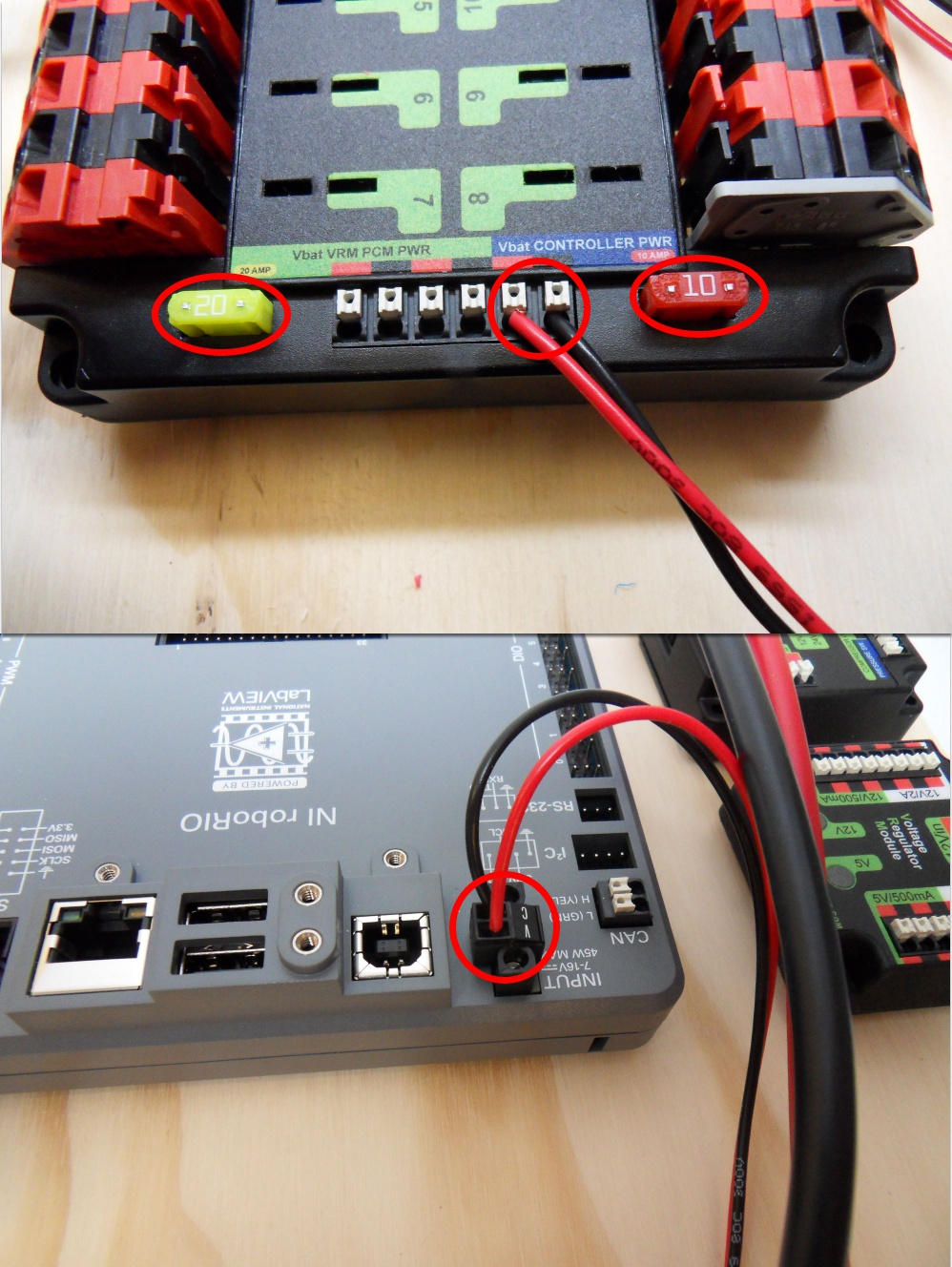
roboRIO Power
Requires: 10A/20A mini fuses, Wire stripper, very small flat screwdriver, 18 AWG (1 \(mm^2\)) Red and Black
Insert the 10A and 20A mini fuses in the PDP in the locations shown on the silk screen (and in the image above)
Strip ~5/16” (~8 mm) on both the red and black 18 AWG (1 \(mm^2\)) wire and connect to the “Vbat Controller PWR” terminals on the PDB
Measure the required length to reach the power input on the roboRIO. Take care to leave enough length to route the wires around any other components such as the battery and to allow for any strain relief or cable management.
Cut and strip the wire.
Using a very small flat screwdriver connect the wires to the power input connector of the roboRIO (red to V, black to C). Also make sure that the power connector is screwed down securely to the roboRIO.
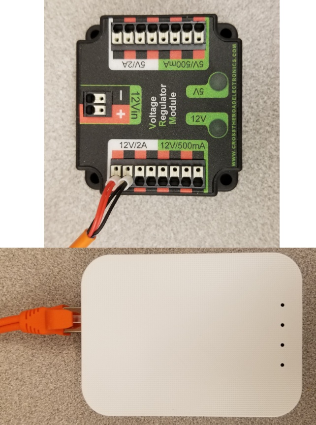
Voltage Regulator Module Power
Requires: Wire stripper, small flat screwdriver (optional), 18 AWG (1 \(mm^2\)) red and black wire:
Strip ~5/16” (~8 mm) on the end of the red and black 18 AWG (1 \(mm^2\)) wire.
Connect the wire to one of the two terminal pairs labeled “Vbat VRM PCM PWR” on the PDP.
Measure the length required to reach the “12Vin” terminals on the VRM. Take care to leave enough length to route the wires around any other components such as the battery and to allow for any strain relief or cable management.
Cut and strip ~5/16” (~8 mm) from the end of the wire.
Connect the wire to the VRM 12Vin terminals.
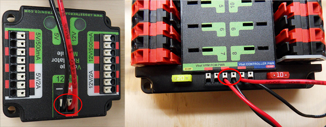
Pneumatics Control Module Power (Optional)
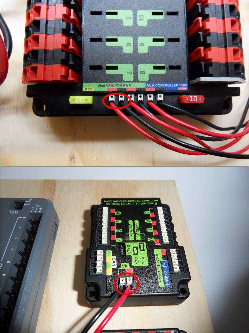
Requires: Wire stripper, small flat screwdriver (optional), 18 AWG (1 \(mm^2\)) red and black wire
Strip ~5/16” (~8 mm) on the end of the red and black 18 AWG (1 \(mm^2\)) wire.
Connect the wire to one of the two terminal pairs labeled “Vbat VRM PCM PWR” on the PDP.
Measure the length required to reach the “Vin” terminals on the PCM. Take care to leave enough length to route the wires around any other components such as the battery and to allow for any strain relief or cable management.
Cut and strip ~5/16” (~8 mm) from the end of the wire.
Connect the wire to the PCM 12Vin terminals.
Radio Power and Ethernet
Warning
DO NOT connect the Rev passive POE injector cable directly to the roboRIO. The roboRIO MUST connect to the female end of the cable using an additional Ethernet cable as shown in the next step.
Requires: Small flat screwdriver (optional), Rev radio PoE cable
Insert the ferrules of the passive PoE injector cable into the corresponding colored terminals on the 12V/2A section of the VRM.
Connect the male RJ45 (Ethernet) end of the cable into the Ethernet port on the radio closest to the barrel connector (labeled 18-24v POE)
roboRIO to Radio Ethernet
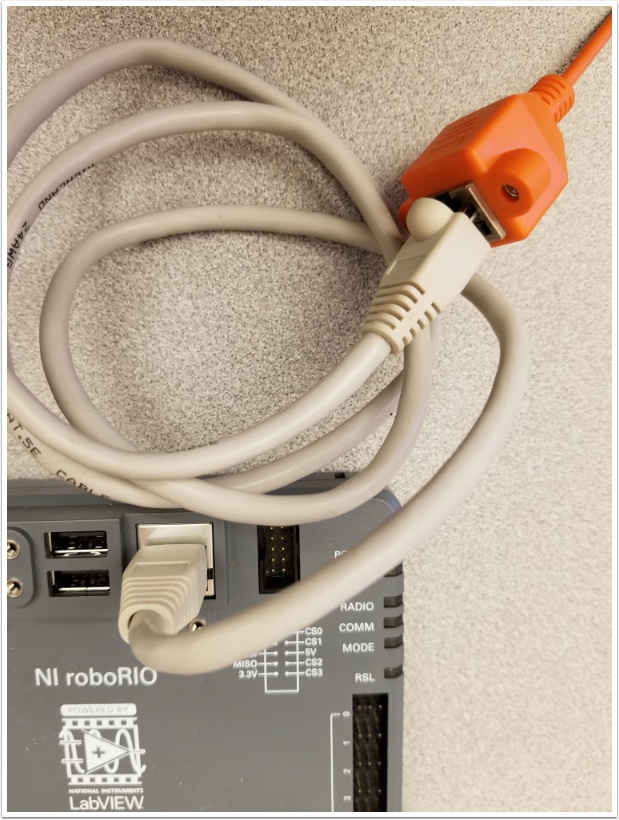
Requires: Ethernet cable
Connect an Ethernet cable from the female RJ45 (Ethernet) port of the Rev Passive POE cable to the RJ45 (Ethernet) port on the roboRIO.
CAN Devices
roboRIO to PCM CAN
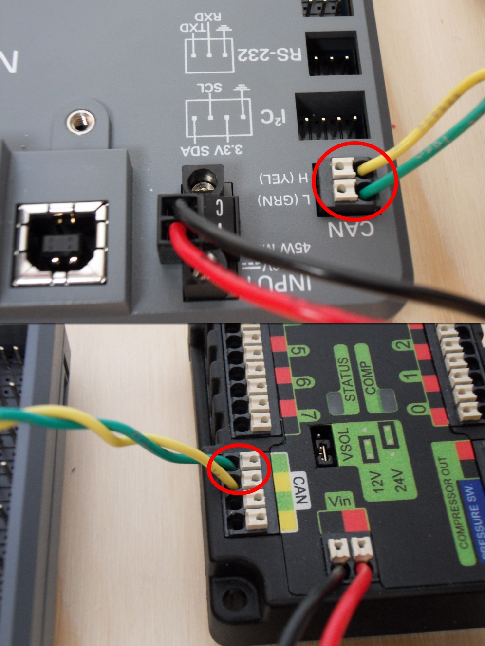
Requires: Wire stripper, small flat screwdriver (optional), yellow/green twisted CAN cable
Strip ~5/16” (~8 mm) off of each of the CAN wires.
Insert the wires into the appropriate CAN terminals on the roboRIO (Yellow->YEL, Green->GRN).
Measure the length required to reach the CAN terminals of the PCM (either of the two available pairs). Cut and strip ~5/16” (~8 mm) off this end of the wires.
Insert the wires into the appropriate color coded CAN terminals on the PCM. You may use either of the Yellow/Green terminal pairs on the PCM, there is no defined in or out.
PCM to PDP CAN
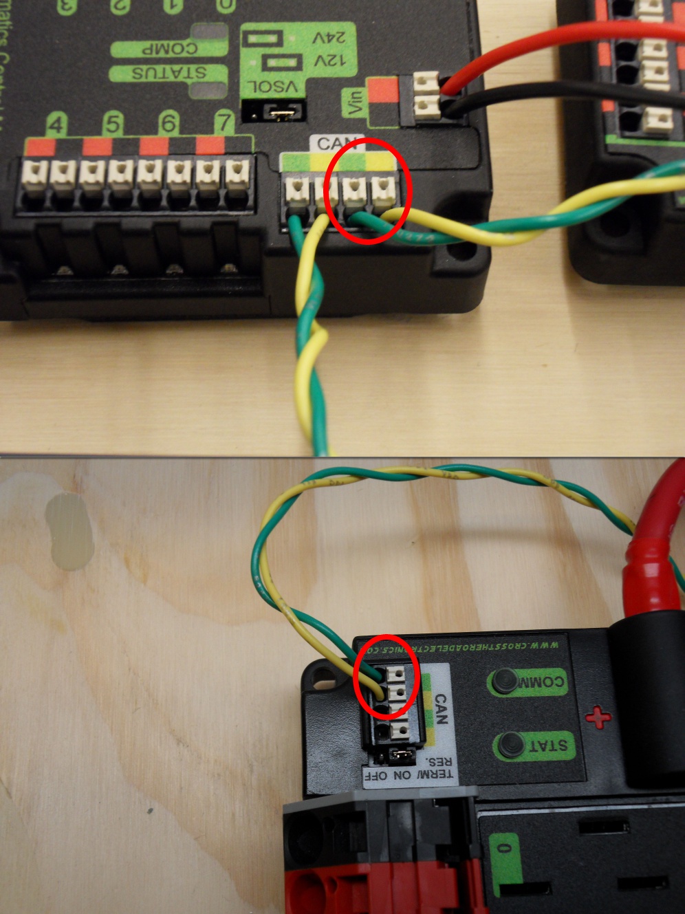
Requires: Wire stripper, small flat screwdriver (optional), yellow/green twisted CAN cable
Strip ~5/16” (~8 mm) off of each of the CAN wires.
Insert the wires into the appropriate CAN terminals on the PCM.
Measure the length required to reach the CAN terminals of the PDP (either of the two available pairs). Cut and strip ~5/16” (~8 mm) off this end of the wires.
Insert the wires into the appropriate color coded CAN terminals on the PDP. You may use either of the Yellow/Green terminal pairs on the PDP, there is no defined in or out.
PWM Cables
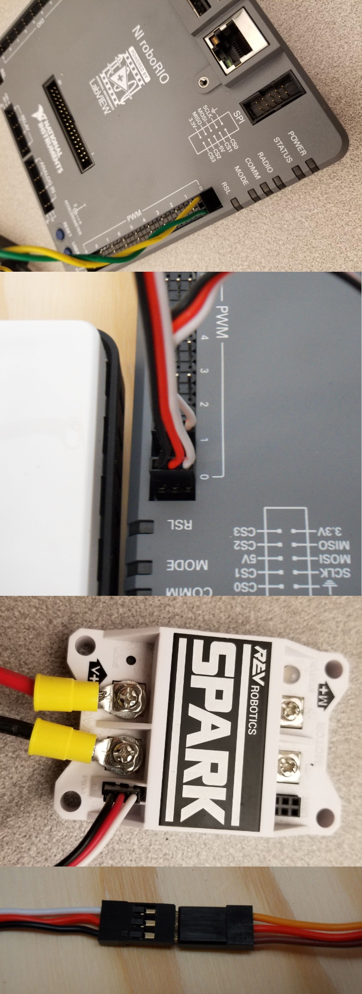
This section details how to wire the SPARK MAX controllers using PWM signaling. This is a recommended starting point as it is less complex and easier to troubleshoot than CAN operation. The SPARK MAXs (and many other FRC motor controllers) can also be wired using CAN which unlocks easier configuration, advanced functionality, better diagnostic data and reduces the amount of wire needed.
Requires: 4x SPARK MAX PWM adapters (if using SPARK MAX), 4x PWM cables (if controllers without integrated wires or adapters, otherwise optional), 2x PWM Y-cable (Optional)
Option 1 (Direct connect):
If using SPARK MAX, attach the PWM adapter to the SPARK MAX (small adapter with a 3 pin connector with black/white wires).
If needed, attach PWM extension cables to the controller or adapter. On the controller side, match the colors or markings (some controllers may have green/yellow wiring, green should connect to black).
Attach the other end of the cable to the roboRIO with the black wire towards the outside of the roboRIO. It is recommended to connect the left side to PWM 0 and 1 and the right side to PWM 2 and 3 for the most straightforward programming experience, but any channel will work as long as you note which side goes to which channel and adjust the code accordingly.
Option 2 (Y-cable):
If using SPARK MAX, attach the PWM adapter to the SPARK MAX (small adapter with a 3 pin connector with black/white wires).
If needed, attach PWM extension cables between the controller or adapter and the PWM Y-cable. On the controller side, match the colors or markings (some controllers may have green/yellow wiring, green should connect to black).
Connect 1 PWM Y-cable to the 2 PWM cables for the controllers controlling each side of the robot. The brown wire on the Y-cable should match the black wire on the PWM cable.
Connect the PWM Y-cables to the PWM ports on the roboRIO. The brown wire should be towards the outside of the roboRIO. It is recommended to connect the left side to PWM 0 and the right side to PWM 1 for the most straightforward programming experience, but any channel will work as long as you note which side goes to which channel and adjust the code accordingly.
Robot Signal Light
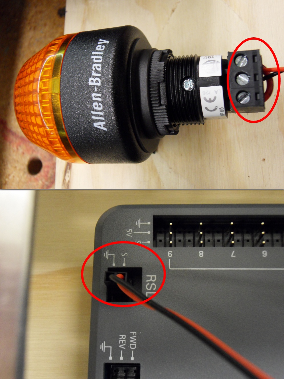
Requires: Wire stripper, 2 pin cable, Robot Signal Light, 18 AWG (1 \(mm^2\)) red wire, very small flat screwdriver
Cut one end off of the 2 pin cable and strip both wires
Insert the black wire into the center, “N” terminal and tighten the terminal.
Strip the 18 AWG (1 \(mm^2\)) red wire and insert into the “La” terminal and tighten the terminal.
Cut and strip the other end of the 18 AWG (1 \(mm^2\)) wire to insert into the “Lb” terminal
Insert the red wire from the two pin cable into the “Lb” terminal with the 18 AWG (1 \(mm^2\)) red wire and tighten the terminal.
Connect the two-pin connector to the RSL port on the roboRIO. The black wire should be closest to the outside of the roboRIO.
Tip
You may wish to temporarily secure the RSL to the control board using cable ties or Dual Lock (it is recommended to move the RSL to a more visible location as the robot is being constructed)
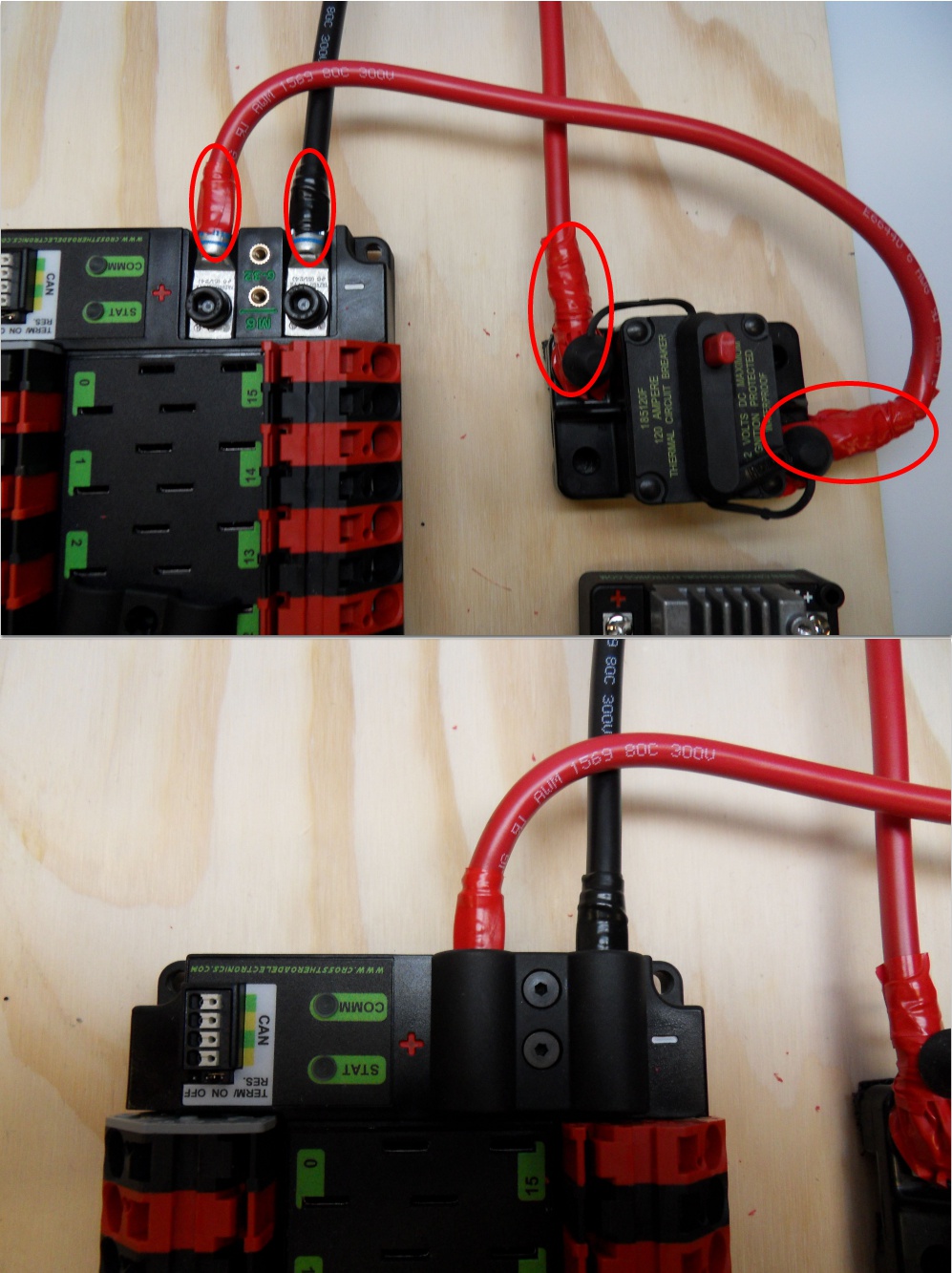
Circuit Breakers
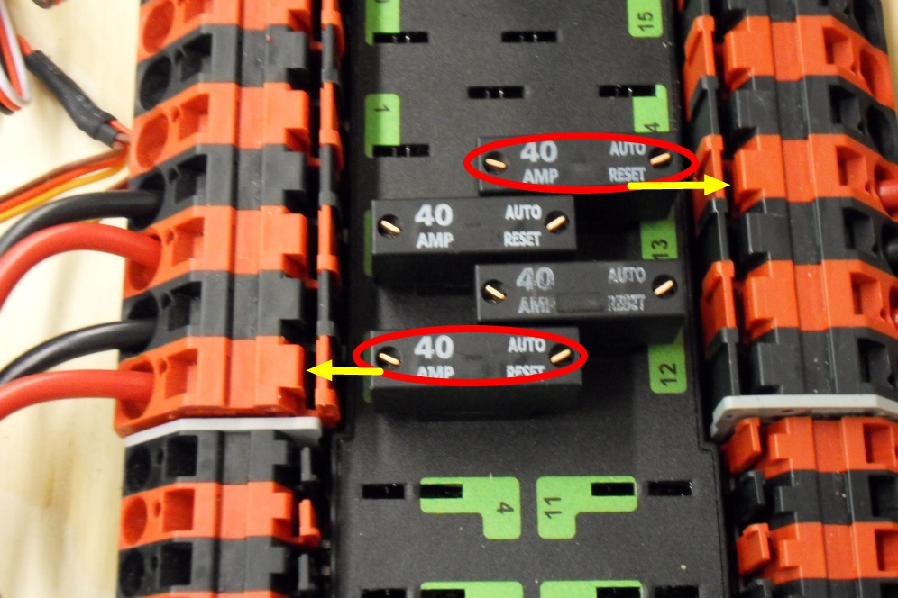
Requires: 4x 40A circuit breakers
Insert 40-amp Circuit Breakers into the positions on the PDP corresponding with the Wago connectors the Talons are connected to. Note that, for all breakers, the breaker corresponds with the nearest positive (red) terminal (see graphic above). All negative terminals on the board are directly connected internally.
If working on a Robot Quick Build, stop here and insert the board into the robot chassis before continuing.
Motor Power
Requires: Wire stripper, wire crimper, phillips head screwdriver, wire connecting hardware
For each CIM motor:
Strip the ends of the red and black wires from the CIM
For integrated wire controllers including SPARK MAX (top image):
Strip the red and black wires (or white and green wires) from the controller (the SPARK MAX white wire is unused for brushed motors such as the CIM, it should be secured and the end should be insulated such with electrical tape or other insulation method).
Connect the motor wires to the matching controller output wires (for controllers with white/green, connect red to white and green to black). The images above show an example using quick disconnect terminals which are provided in the Rookie KOP.
For the SPARK or other non-integrated-wire controllers (bottom image):
Crimp a ring/fork terminal on each of the motor wires.
Attach the wires to the output side of the motor controller (red to +, black to -)
STOP

Danger
Before plugging in the battery, make sure all connections have been made with the proper polarity. Ideally have someone that did not wire the robot check to make sure all connections are correct.
Before plugging in the battery, make sure all connections have been made with the proper polarity. Ideally have someone that did not wire the robot check to make sure all connections are correct.
Start with the battery and verify that the red wire is connected to the positive terminal
Check that the red wire passes through the main breaker and to the + terminal of the PDP and that the black wire travels directly to the - terminal.
For each motor controller, verify that the red wire goes from the red PDP terminal to the Red wire on the Victor SPX (not the white M+!!!!)
For each device on the end of the PDP, verify that the red wire connects to the red terminal on the PDP and the red terminal on the component.
Make sure that the orange Passive PoE cable is plugged directly into the radio NOT THE roboRIO! It must be connected to the roboRIO using an additional Ethernet cable.
Tip
It is also recommended to put the robot on blocks so the wheels are off the ground before proceeding. This will prevent any unexpected movement from becoming dangerous.
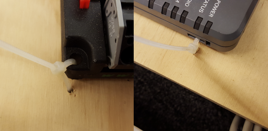
Manage Wires
Requires: Zip ties
Tip
Now may be a good time to add a few zip ties to manage some of the wires before proceeding. This will help keep the robot wiring neat.
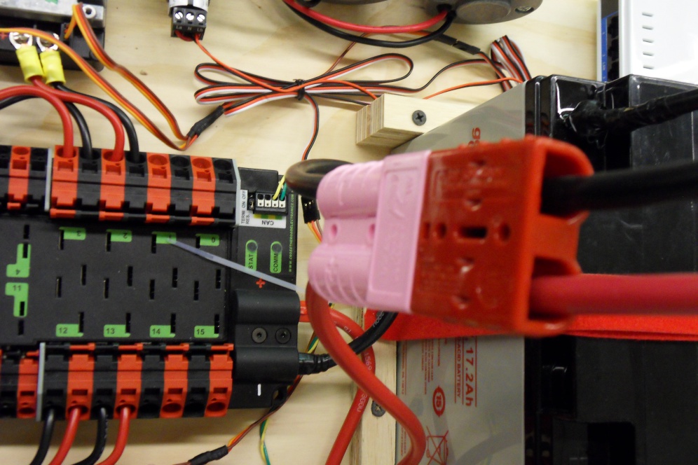
Connect Battery
Connect the battery to the robot side of the Anderson connector. Power on the robot by moving the lever on the top of the 120A main breaker into the ridge on the top of the housing.
If stuff blinks, you probably did it right.
Before moving on, if using SPARK MAX controllers, there is one more configuration step to complete. The SPARK MAX motor controllers are configured to control a brushless motor by default. You can verify this by checking that the light on the controller is blinking either cyan or magenta (indicating brushless brake or brushless coast respectively). To change to to brushed mode, press and hold the mode button for 3-4 seconds until the status LED changes color. The LED should change to either blue or yellow, indicating that the controller is in brushed mode (brake or coast respectively). To change the brake or coast mode, which control how quickly the motor slows down when a neutral signal is applied, press the mode button briefly.
Tip
For more information on the SPARK MAX motor controllers, including how to test your motors/controllers without writing any code by using the REV Hardware Client, see the SPARK MAX Quickstart guide.
From here, you should connect to the roboRIO and try uploading your code!
Step 2: Installing Software
An overview of the available control system software can be found here.
Offline Installation Preparation
This article contains instructions/links to components you will want to gather if you need to do offline installation of the FRC® Control System software.
Tip
This document compiles all the download links from the following documents to make it easier to install on offline computers or on multiple computers. If you are you installing on a single computer that is connected to the internet, you can skip this page.
Note
The order in which these tools are installed does not matter for Java and C++ teams. LabVIEW should be installed before the FRC Game Tools or 3rd Party Libraries.
Documentation
This documentation can be downloaded for offline viewing. The link to download the PDF can be found here.
Installers
All Teams
2022 FRC Game Tools (Note: Click on link for “Individual Offline Installers”)
2022 FRC Radio Configuration Utility or 2022 FRC Radio Configuration Utility Israel Version
(Optional - Veterans Only!) Classmate/Acer PC Image
LabVIEW Teams
LabVIEW USB (from FIRST® Choice) or Download (Note: Click on link for “Individual Offline Installers”)
Java/C++ Teams
Note
After downloading the Java/C++ WPILib installer, run it once while connected to the internet and select Install for this User then Create VS Code zip to share with other computers/OSes for offline install and save the downloaded VS Code zip file for future offline installations.
3rd Party Libraries/Software
A directory of available 3rd party software that plugs in to WPILib can be found on 3rd Party Libraries.
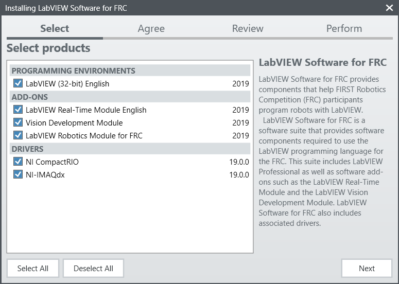
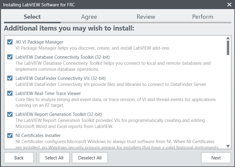
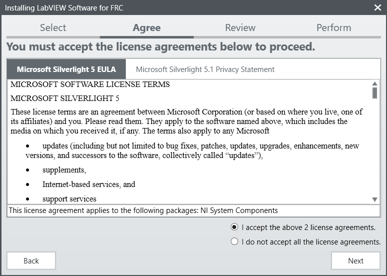
Installing LabVIEW for FRC (LabVIEW only)
Note
This installation is for teams programming in LabVIEW or using NI Vision Assistant only. C++ and Java teams not using these features do not need to install LabVIEW and should proceed to Installing the FRC Game Tools.
Download and installation times will vary widely with computer and internet connection specifications, however note that this process involves a large file download and installation and will likely take at least an hour to complete.
Requirements
Windows 10 or higher (Windows 10, 11). Windows 11 is not officially supported by NI, but has been tested to work.
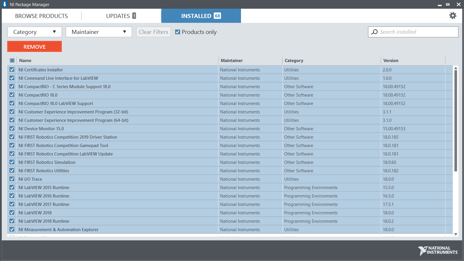
Uninstall Old Versions (Recommended)
Note
If you wish to keep programming cRIOs you will need to maintain an install of LabVIEW for FRC® 2014. The LabVIEW for FRC 2014 license has been extended. While these versions should be able to co-exist on a single computer, this is not a configuration that has been extensively tested.
Before installing the new version of LabVIEW it is recommended to remove any old versions. The new version will likely co-exist with the old version, but all testing has been done with FRC 2020 only. Make sure to back up any team code located in the “User\LabVIEW Data” directory before un-installing. Then click Start >> Add or Remove Programs. Locate the entry labeled “National Instruments Software” or “NI Software”, and select Uninstall.
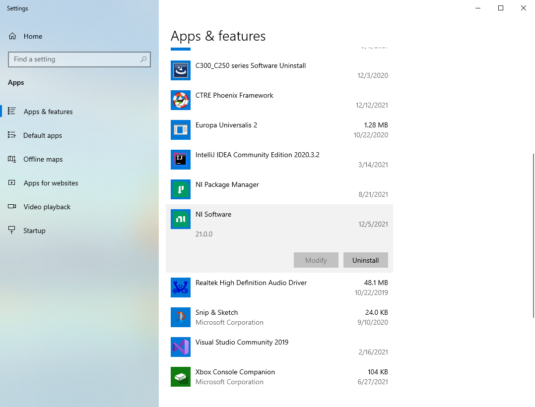
Select Components to Uninstall
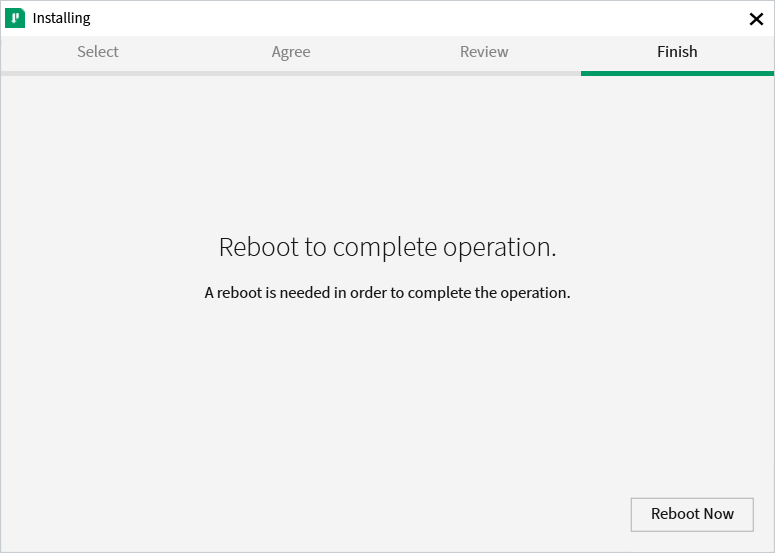
In the dialog box that appears, select all entries. The easiest way to do this is to de-select the “Products Only” check-box and select the check-box to the left of “Name”. Click Remove. Wait for the uninstaller to complete and reboot if prompted.
Warning
These instructions assume that no other NI software is installed. If you have other NI software installed, it is necessary to uncheck the software that should not be uninstalled.
Getting LabVIEW installer
Either locate and insert the LabVIEW USB Drive or download the LabVIEW for FRC 2020 installer from NI. Be sure to select the correct version from the drop-down.
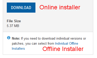
If you wish to install on other machines offline, do not click the Download button, click Individual Offline Installers and then click Download, to download the full installer.
Note
This is a large download (~8GB). It is recommended to use a fast internet connection and to use the NI Downloader to allow the download to resume if interrupted.
Installing LabVIEW
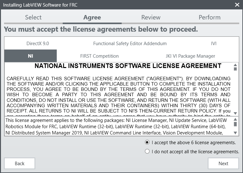
NI LabVIEW requires a license. Each season’s license is active until January 31st of the following year (e.g. the license for the 2020 season expires on January 31, 2021)
Teams are permitted to install the software on as many team computers as needed, subject to the restrictions and license terms that accompany the applicable software, and provided that only team members or mentors use the software, and solely for FRC. Rights to use LabVIEW are governed solely by the terms of the license agreements that are shown during the installation of the applicable software.
Starting Install
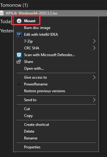
Run the downloaded exe file to start the install process. Click Yes if a Windows Security prompt
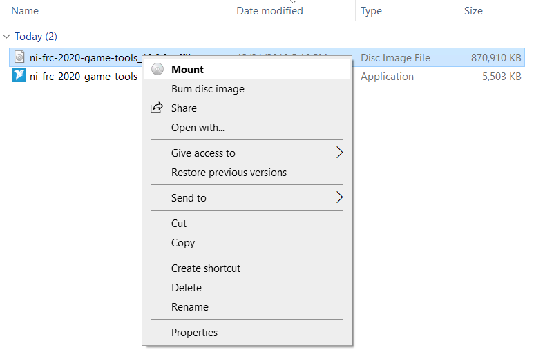
Right click on the downloaded iso file and select mount. Run install.exe from the mounted iso. Click “Yes” if a Windows Security prompt
Note
other installed programs may associate with iso files and the mount option may not appear. If that software does not give the option to mount or extract the iso file, then install 7-Zip and use that to extract the iso.
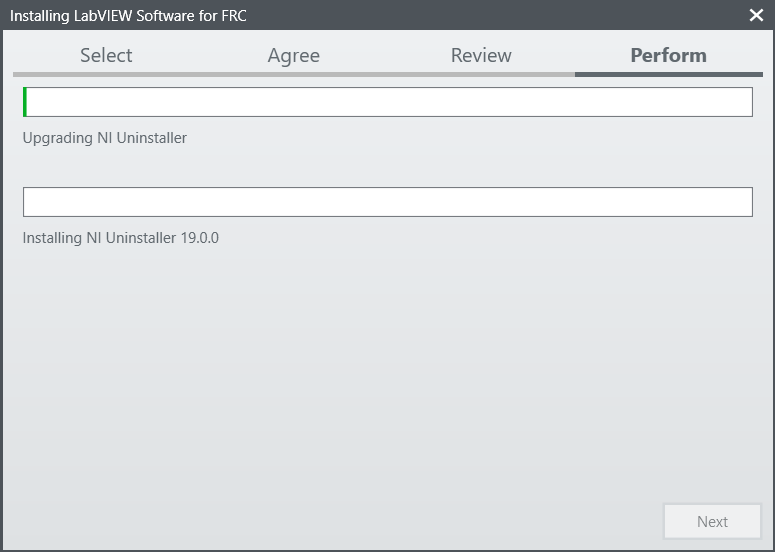
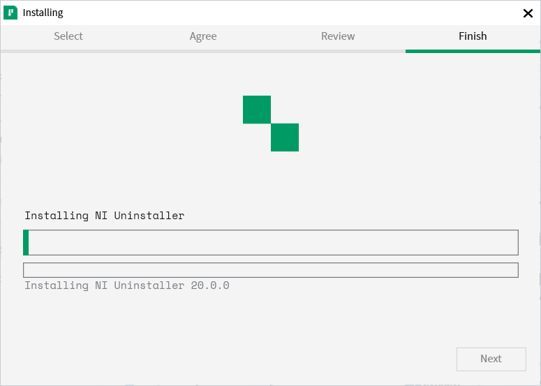
NI Package Manager Installation
Installation progress of the NI Package Manager will be tracked in this window

NI Update Service
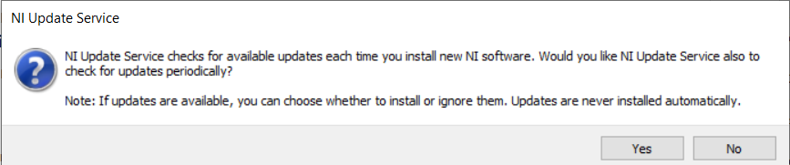
You will be prompted whether to enable the NI update service. You can choose to not enable the update service.
Warning
It is not recommended to install these updates unless directed by FRC through our usual communication channels (FRC Blog, Team Updates or E-mail Blasts).
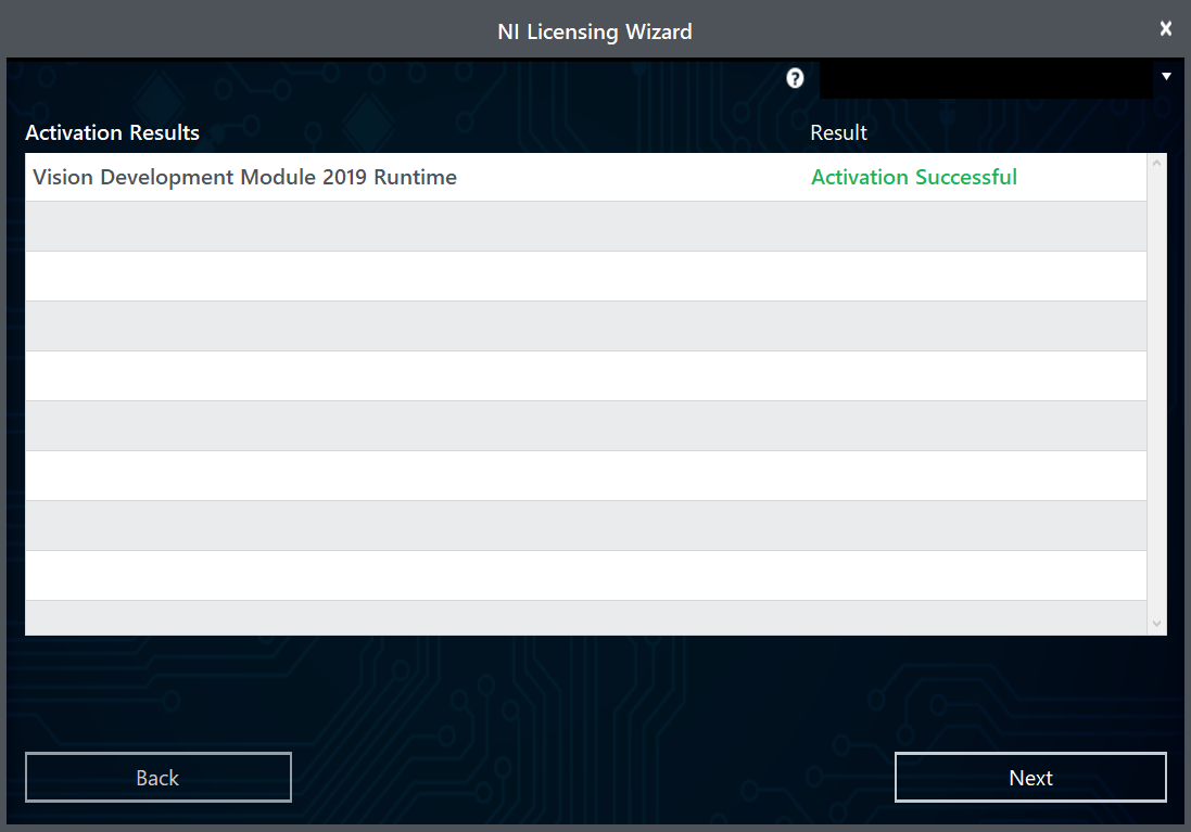
NI Activation Wizard
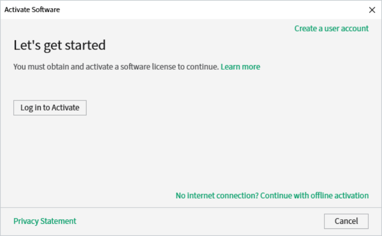
Click the Log in to Activate button.
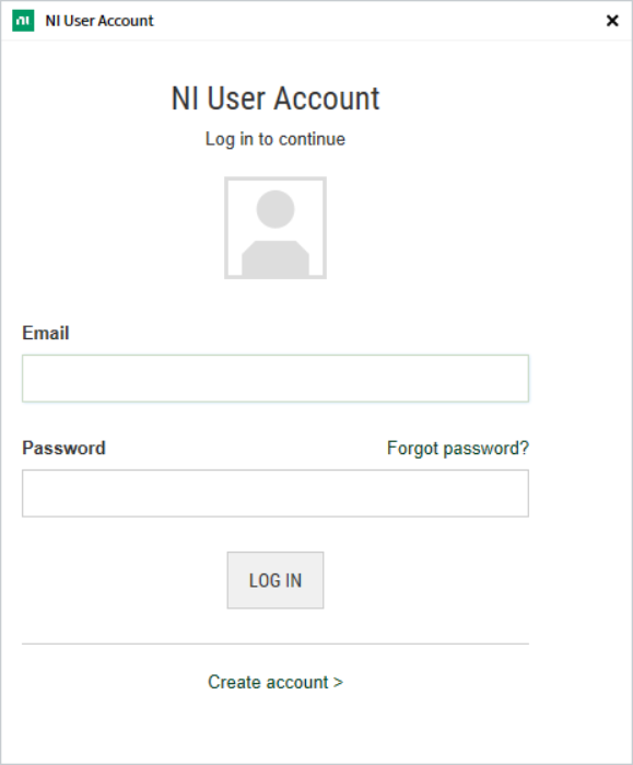
Log into your ni.com account. If you don’t have an account, select Create account to create a free account.
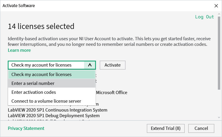
From the drop-down, select enter a serial number
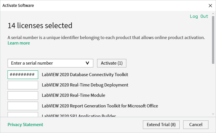
Enter the serial number in all the boxes. Click Activate.
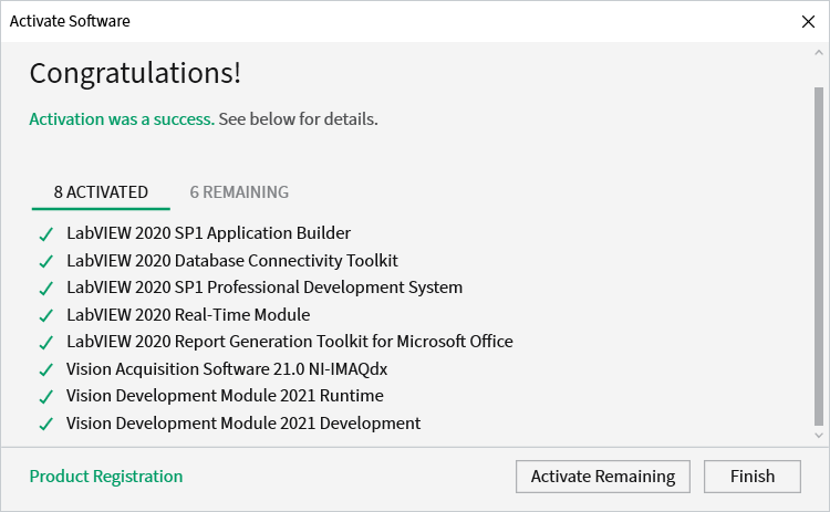
If your products activate successfully, an “Activation Successful” message will appear. If the serial number was incorrect, it will give you a text box and you can re-enter the number and select Try Again. The items shown above are not expected to activate. If everything activated successfully, click Finish.
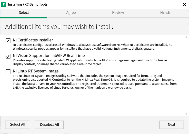
Installing the FRC Game Tools
The FRC® Game Tools contains the following software components:
LabVIEW Update
FRC Driver Station
FRC Utilities
The LabVIEW runtime components required for the Driver Station and Utilities are included in this package.
Note
No components from the LabVIEW Software for FRC package are required for running either the Driver Station or Utilities.
Requirements
Windows 10 or higher (Windows 10, 11). Windows 11 is not officially supported by NI, but has been tested to work.
Download the FRC Game Tools from NI.
If you wish to install on other machines offline, click Individual Offline Installers before clicking Download to download the full installer.
Uninstall Old Versions (Recommended)
Important
LabVIEW teams have already completed this step, do not repeat it. LabVIEW teams should skip to the Installation section.
Before installing the new version of the FRC Game Tools it is recommended to remove any old versions. The new version will likely co-exist with the old version (note that the DS will overwrite old versions), but all testing has been done with FRC 2022 only. Then click Start >> Add or Remove Programs. Locate the entry labeled “National Instruments Software” or “NI Software”, and select Uninstall.
Note
It is only necessary to uninstall previous versions when installing a new year’s tools. For example, uninstall the 2021 tools before installing the 2022 tools. It is not necessary to uninstall before upgrading to a new update of the 2022 game tools.
Select Components to Uninstall
In the dialog box that appears, select all entries. The easiest way to do this is to de-select the Products Only check-box and select the check-box to the left of “Name”. Click Remove. Wait for the uninstaller to complete and reboot if prompted.
Installation
Important
The Game Tools installer may prompt that .NET Framework 4.6.2 needs to be updated or installed. Follow prompts on-screen to complete the installation, including rebooting if requested. Then resume the installation of the FRC Game Tools, restarting the installer if necessary.
Extraction
Run the downloaded executable file to start the install process. Click Yes if a Windows Security prompt appears.
Right click on the downloaded iso file and select mount. Run install.exe from the mounted iso. Click Yes if a Windows Security prompt appears.
Note
Other installed programs may associate with iso files and the mount option may not appear. If that software does not give the option to mount or extract the iso file, then install 7-Zip and use that to extract the iso.
NI Package Manager License
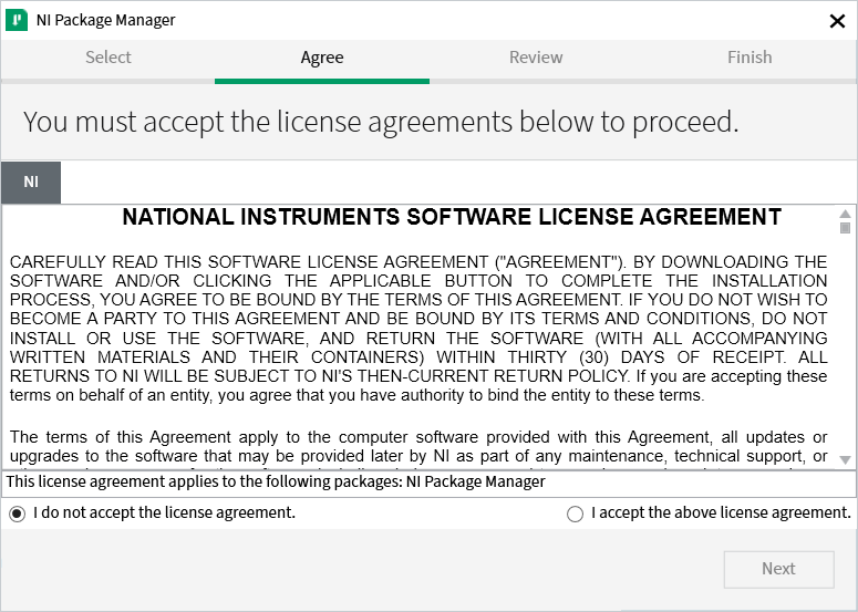
If you see this screen, click Next. This screen confirms that you agree to NI Package Manager License agreement.
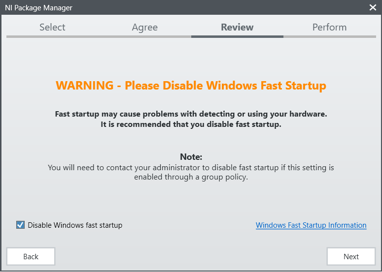
Disable Windows Fast Startup
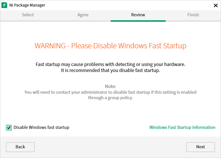
It is recommended to leave this screen as-is, as Windows Fast Startup can cause issues with the NI drivers required to image the roboRIO. Go ahead and click Next.
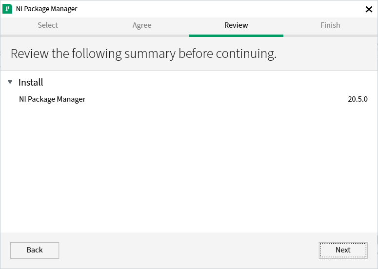
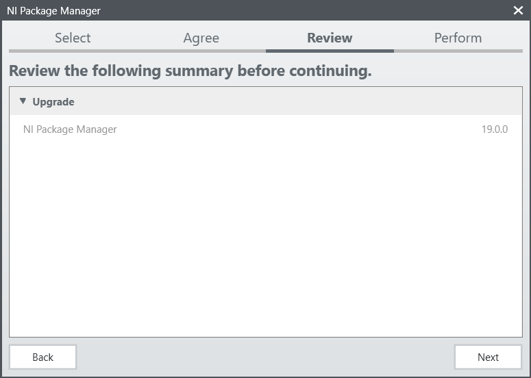
NI Package Manager Installation
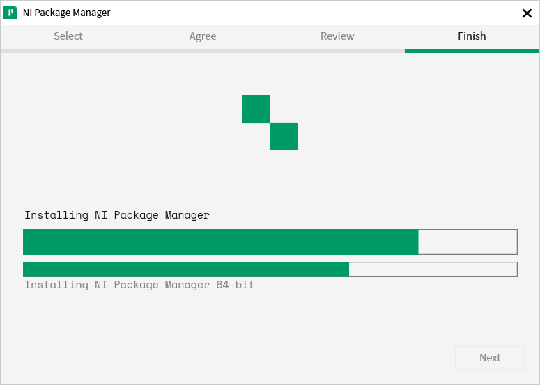
Installation progress of the NI Package Manager will be tracked in this window.
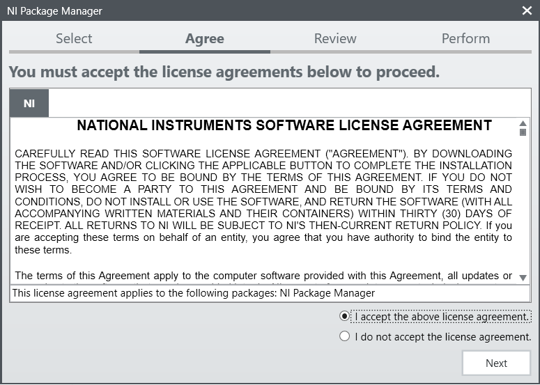
License Agreements
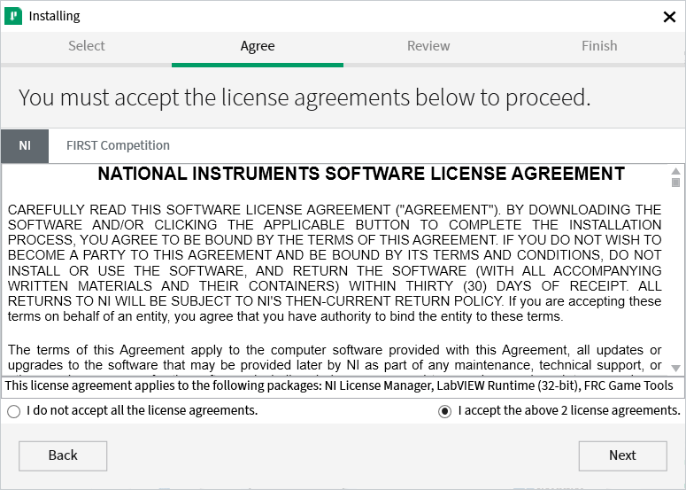
Select I accept… then click Next
Go ahead and press I accept… then click Next, confirming that you agree to the NI License agreement.

Detail Progress
This screen showcases the installation process, go ahead and press Next when it’s finished.
NI Activation Wizard
Log into your ni.com account. If you don’t have an account, select Create account to create a free account.
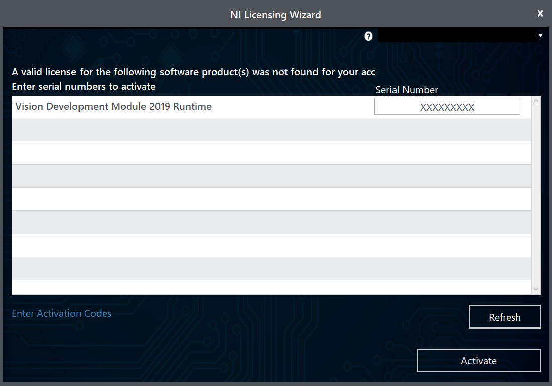
Enter the serial number. Click Activate.
Note
If this is the first time activating this year’s software on this account, you will see the message shown above about a valid license not being found. You can ignore this.
If your products activate successfully, an Activation Successful message will appear. If the serial number was incorrect, it will give you a text box and you can re-enter the number and select Try Again. If everything activated successfully, click Next.
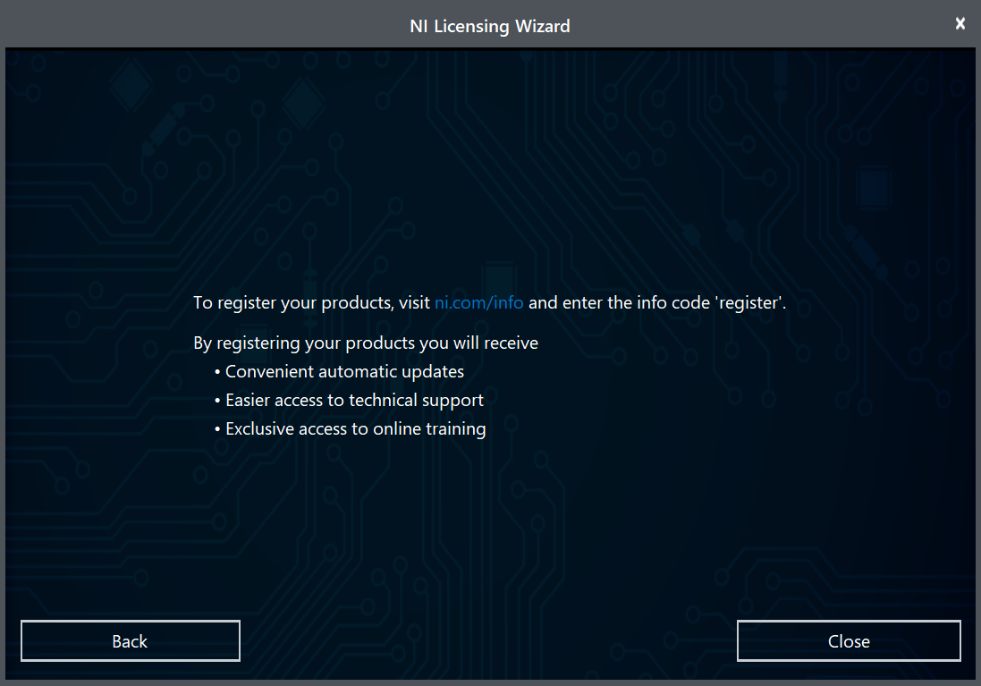
Click Close.
NI Update Service
You will be prompted whether to enable the NI update service. You can choose to not enable the update service.
Warning
It is not recommended to install these updates unless directed by FRC through our usual communication channels (FRC Blog, Team Updates or E-mail Blasts).
WPILib Installation Guide
This guide is intended for Java and C++ teams. LabVIEW teams can skip to Installing LabVIEW for FRC (LabVIEW only). Additionally, the below tutorial shows Windows 10, but the steps are identical for all operating systems. Notes differentiating operating systems will be shown.
Prerequisites
You can download the latest release of the installer from GitHub. Ensure that you download the correct binary for your OS and architecture.
Warning
Windows 7 users must have an updated system with this update installed. MacOS and Linux require python3 installed.
Warning
The following OSes will be unsupported starting 2023: Ubuntu 18.04, Windows 7, Windows 8.1, and any 32-bit Windows. MacOS 10.14 is no longer supported as of 2022.
WPILib is designed to install to different folders for different years, so that it is not necessary to uninstall a previous version before installing this year’s WPILib.
Extracting the Installer
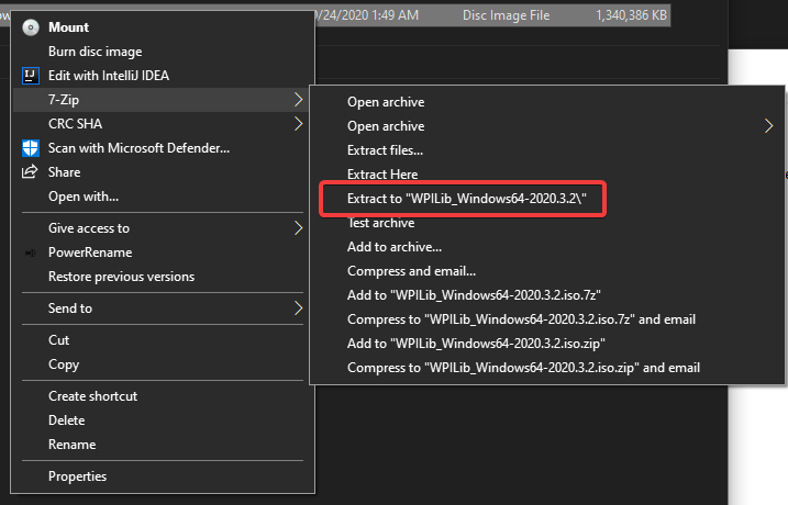
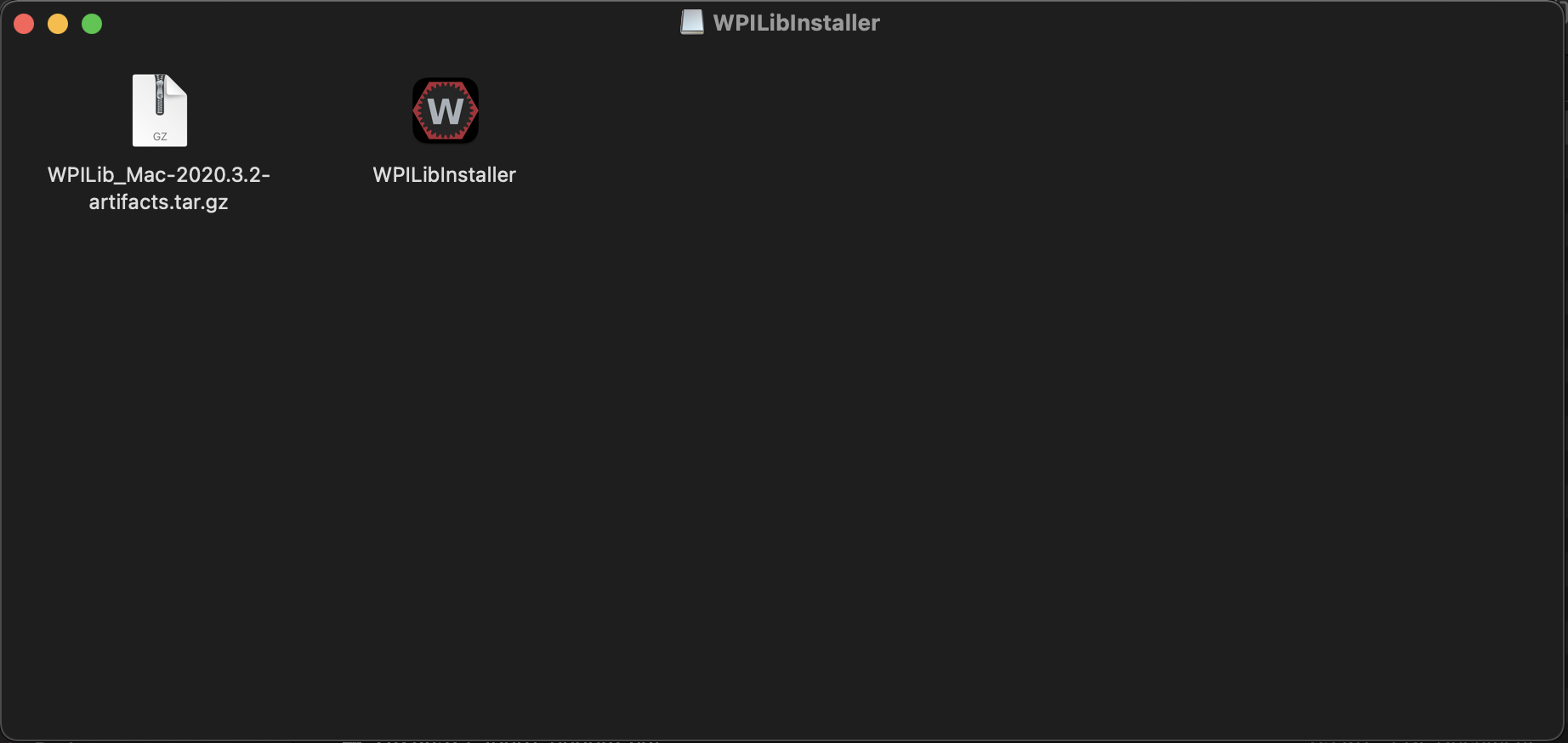
When you download the WPILib installer, it is distributed as a disk image file .iso for Windows, .tar.gz for Linux, and distributed as a DMG for MacOS.
Note
Other installed programs may associate with iso files and the mount option may not appear. If that software does not give the option to mount or extract the iso file, then follow the directions in the “Windows 7” tab.
You can use 7-zip to extract the disk image by right-clicking, selecting 7-Zip and selecting Extract to…. Then launch WPILibInstaller.exe
macOS users can double click on the downloaded DMG and then select WPILibInstaller to launch the application.
Linux users should extract the downloaded .tar.gz and then launch WPILibInstaller. Ubuntu treats executables in the file explorer as shared libraries, so double-clicking won’t run them. Run the following commands in a terminal instead with <version> replaced with the version you’re installing.
$ tar -xf WPILib_Linux-<version>.tar.gz
$ cd WPILib_Linux-<version>/
$ ./WPILibInstaller
Running the Installer
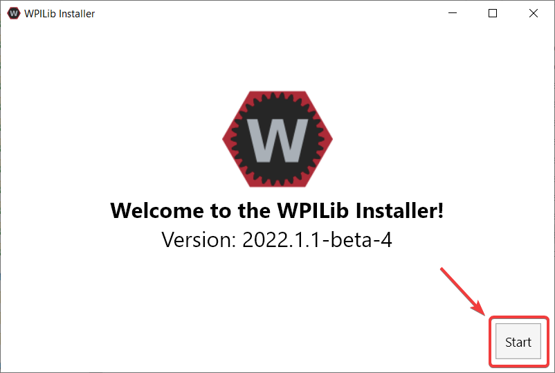
Upon opening the installer, you’ll be presented with the below screen. Go ahead and press Start.
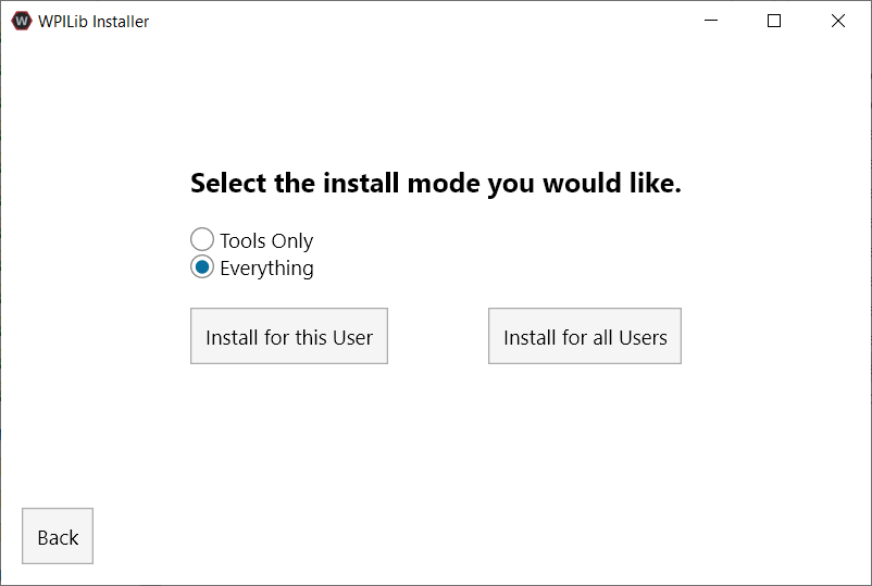
This showcases a list of options included with the WPILib installation.
Tools Only installs just the WPILib tools (Pathweaver, Shuffleboard, RobotBuilder, SysID, Glass, and OutlineViewer) and JDK.
Everything installs the full development environment (VS Code, extensions, all dependencies), WPILib tools, and JDK.
You will notice two buttons, Install for this User and Install for all Users. Install for this User only installs it on the current user account, and does not require administrator privileges. However, Install for all Users installs the tools for all system accounts and will require administrator access. Install for all Users is not an option for macOS and Linux.
Note
If you select Install for all Users, Windows will prompt for administrator access through UAC during installation.
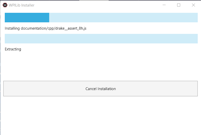
Select the option that is appropriate for you, and you’ll presented with the following installation screen.
This next screen involves downloading VS Code. Unfortunately, due to licensing reasons, VS Code can not be bundled with the installer.
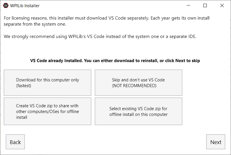
Download for this computer only
This downloads VS Code only for the current platform, which is also the smallest download.
Skip and don’t use VS Code
Skips installing VS Code. Useful for advanced installations or configurations. Generally not recommended.
Select existing VS Code zip for offline install on this computer
Selecting this option will bring up a prompt allowing you to select a pre-existing zip file of VS Code that has been downloaded by the installer previously. This option does not let you select an already installed copy of VS Code on your machine.
Create VS Code zip to share with other computers/OSes for offline install
This option downloads and saves a copy of VS Code for all platforms, which is useful for sharing the copy of the installer.
Go ahead and select Download VS Code for Single Install. This will begin the download process and can take a bit depending on internet connectivity (it’s ~100MB). Once the download is done, select Next. You should be presented with a screen that looks similar to the one below.
After installation is complete, you will be presented with the finished screen.
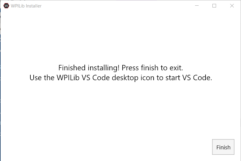
Important
WPILib installs a separate version of VS Code. It does not use an already existing installation. Each year has it’s own copy of the tools appended with the year. IE: WPILib VS Code 2022. Please launch the WPILib VS Code and not a system installed copy!
Congratulations, the WPILib development environment and tooling is now installed on your computer! Press Finish to exit the installer.
Post-Installation
Some operating systems require some final action to complete installation.
After installation, the installer opens the WPILib VS Code folder. Drag the VS Code application to the dock. Eject WPILibInstaller image from the desktop.
Some versions of Linux (e.g. Ubuntu 20.04) require you to give the desktop shortcut the ability to launch. Right click on the desktop icon and select Allow Launching.
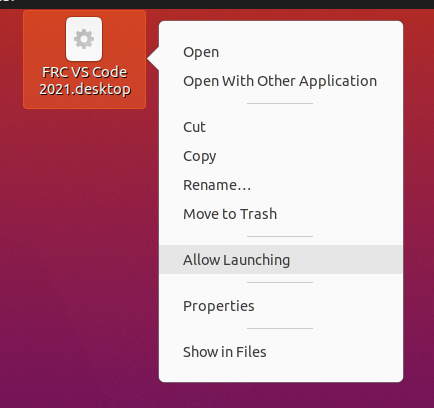
Note
Installing desktop tools and rebooting will create a folder on the desktop called YYYY WPILib Tools, where YYYY is the current year. Desktop tool shortcuts are not available on Linux and MacOS.
Additional C++ Installation for Simulation
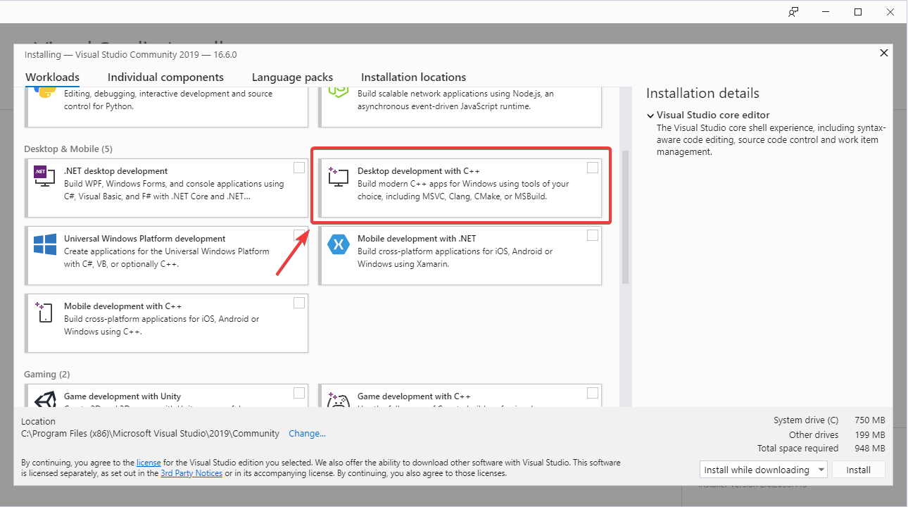
C++ robot simulation requires that a native compiler to be installed. For Windows, this would be Visual Studio 2022 or 2019 (not VS Code), macOS requires Xcode, and Linux (Ubuntu) requires the build-essential package.
Ensure the Desktop Development with C++ option is checked in the Visual Studio installer for simulation support.
What is Installed?
The Offline Installer installs the following components:
Visual Studio Code - The supported IDE for 2019 and later robot code development. The offline installer sets up a separate copy of VS Code for WPILib development, even if you already have VS Code on your machine. This is done because some of the settings that make the WPILib setup work may break existing workflows if you use VS Code for other projects.
C++ Compiler - The toolchains for building C++ code for the roboRIO
Gradle - The specific version of Gradle used for building/deploying C++ or Java robot code
Java JDK/JRE - A specific version of the Java JDK/JRE that is used to build Java robot code and to run any of the Java based Tools (Dashboards, etc.). This exists side by side with any existing JDK installs and does not overwrite the JAVA_HOME variable
WPILib Tools - SmartDashboard, Shuffleboard, RobotBuilder, Outline Viewer, Pathweaver, Glass, SysID
WPILib Dependencies - OpenCV, etc.
VS Code Extensions - WPILib extensions for robot code development in VS Code
Uninstalling
WPILib is designed to install to different folders for different years, so that it is not necessary to uninstall a previous version before installing this year’s WPILib. However, the following instructions can be used to uninstall WPILib if desired.
Delete the appropriate wpilib folder (2019:
c:\Users\Public\frc2019, 2020 and later:c:\Users\Public\wpilib\YYYYwhereYYYYis the year to uninstall)Delete the desktop icons at
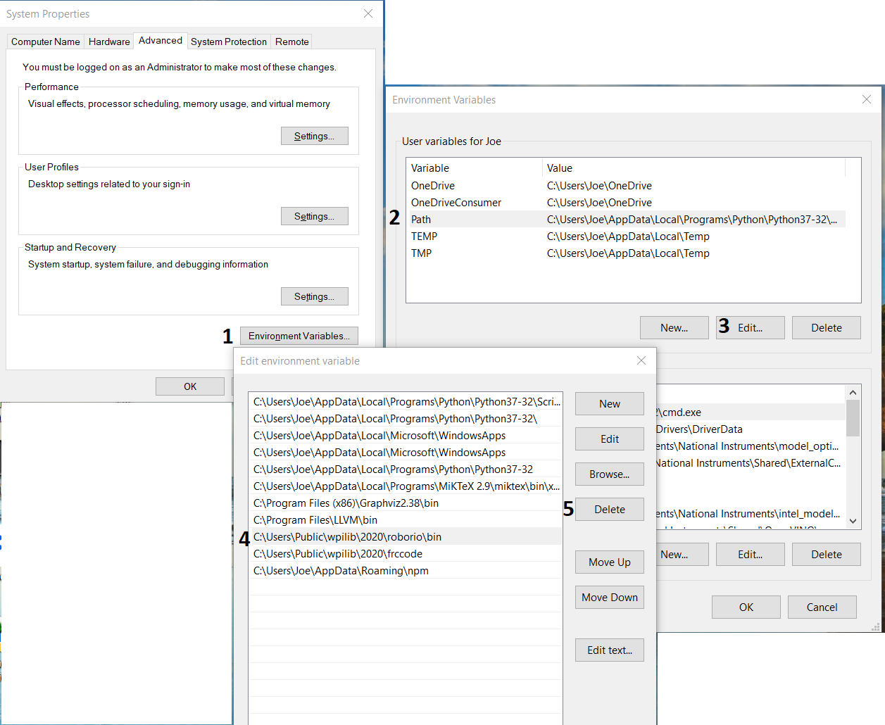
C:\Users\Public\Public DesktopDelete the path environment variables.
In the start menu, type environment and select “edit the system environment variables”
Click on the environment variables button (1).
In the user variables, select path (2) and then click on edit (3).
Select the path with
roborio\bin(4) and click on delete (5).Select the path with
frccodeand click on delete (5).Repeat steps 3-6 in the Systems Variable pane.
Delete the appropriate wpilib folder (2019:
~/frc2019, 2020 and later:~/wpilib/YYYYwhereYYYYis the year to uninstall)
Delete the appropriate wpilib folder (2019:
~/frc2019, 2020 and later:~/wpilib/YYYYwhereYYYYis the year to uninstall). egrm -rf ~/wpilib/YYYY
Next Steps
Congratulations! You have completed step 2 and should now have a working software development environment! Step 3 of this tutorial covers updating the hardware so that you can program it, while Step 4 showcases programming a robot in the VS Code Integrated Development Environment (IDE). For further information you can read through the VS Code section to familiarize yourself with the IDE.
Specific articles that are advised to be read are:
Additionally, you may need to do extra configuration that is applicable to your team’s robot. Please utilize the search feature to find necessary documentation.
Note
It’s important that teams using 3rd-party CAN motor controllers look at the Installing 3rd Party Libraries article as extra steps are required to code for these devices.
Step 3: Preparing Your Robot
Warning
The CAN Web Dashboard plugin is no longer supported by the roboRIO Web Dashboard. To configure CTRE CAN devices such as the PCM and PDP, use CTRE Phoenix Tuner
Imaging your roboRIO
Warning
Before imaging your roboRIO, you must have completed installation of the FRC Game Tools. You also must have the roboRIO power properly wired to the Power Distribution Panel. Make sure the power wires to the roboRIO are secure and that the connector is secure firmly to the roboRIO (4 total screws to check).
Important
The first time a roboRIO 2 is imaged (or if the microSD card is replaced with a new card), it must be imaged using roboRIO 2.0 microSD card imaging process.
Configuring the roboRIO
The roboRIO Imaging Tool will be used to image your roboRIO with the latest software.
USB Connection

Connect a USB cable from the roboRIO USB Device port to the PC. This requires a USB Type A male (standard PC end) to Type B male cable (square with 2 cut corners), most commonly found as a printer USB cable.
Note
The roboRIO should only be imaged via the USB connection. It is not recommended to attempt imaging using the Ethernet connection.
Driver Installation
The device driver should install automatically. If you see a “New Device” pop-up in the bottom right of the screen, wait for the driver install to complete before continuing.
Launching the Imaging Tool
The roboRIO imaging tool and latest image are installed with the NI FRC® Game Tools. Launch the imaging tool by double clicking on the shortcut on the Desktop. If you have difficulties imaging your roboRIO, you may need to try right-clicking on the icon and selecting Run as Administrator instead.
Note
The roboRIO imaging tool is also located at C:\Program Files (x86)\National Instruments\LabVIEW YYYY\project\roboRIO Tool where YYYY is the current year - 1. If it’s 2020, the directory would be LabVIEW 2019.
roboRIO Imaging Tool
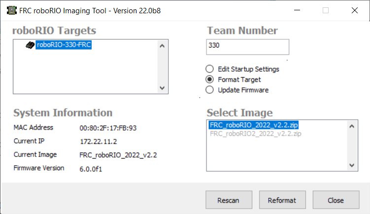
After launching, the roboRIO Imaging Tool will scan for available roboRIOs and indicate any found in the top left box. The bottom left box will show information and settings for the roboRIO currently selected. The right hand pane contains controls for modifying the roboRIO settings:
Edit Startup Settings - This option is used when you want to configure the startup settings of the roboRIO (the settings in the right pane), without imaging the roboRIO.
Format Target - This option is used when you want to load a new image on the roboRIO (or reflash the existing image). This is the most common option.
Update Firmware - This option is used to update the roboRIO firmware. For this season, the imaging tool will require roboRIO firmware to be version 5.0 or greater.
Updating Firmware
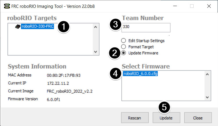
roboRIO firmware must be at least v5.0 to work with the 2019 or later image. If your roboRIO is at least version 5.0 (as shown in the bottom left of the imaging tool) you do not need to update.
To update roboRIO firmware:
Make sure your roboRIO is selected in the top left pane.
Select Update Firmware in the top right pane
Enter a team number in the Team Number box
Select the latest firmware file in the bottom right
Click the Update button
Imaging the roboRIO
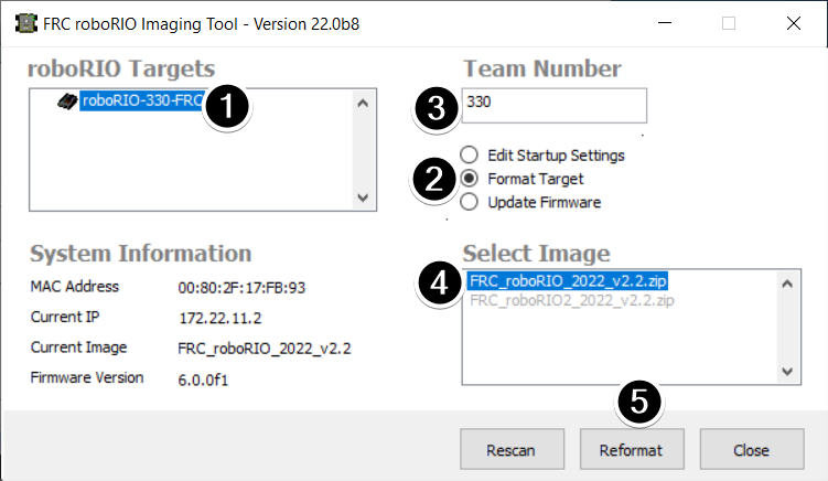
Make sure the roboRIO is selected in the top left pane
Select Format Target in the right pane
Enter your team number in the box
Select the latest image version in the box.
Click Reformat to begin the imaging process.
Imaging Progress
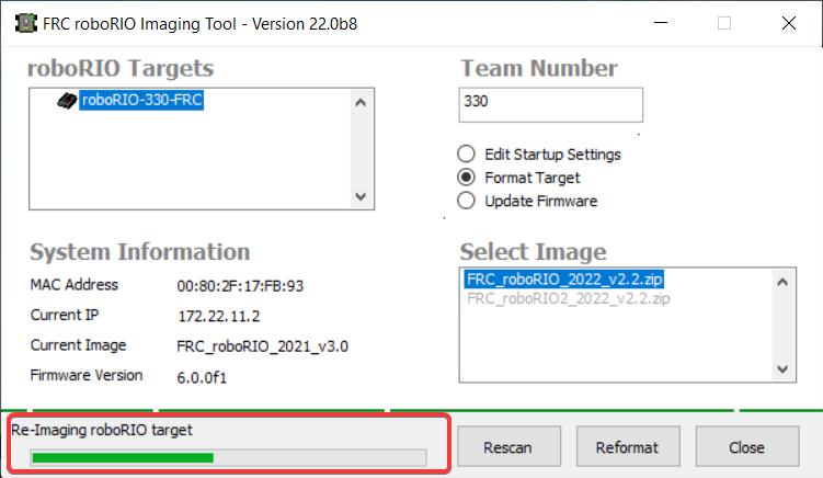
The imaging process will take approximately 3-10 minutes. A progress bar in the bottom left of the window will indicate progress.
Imaging Complete
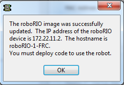
When the imaging completes you should see the dialog above. Click Ok, then click the Close button at the bottom right to close the imaging tool. Reboot the roboRIO using the Reset button to have the new team number take effect.
Troubleshooting
If you are unable to image your roboRIO, troubleshooting steps include:
Try running the roboRIO Imaging Tool as Administrator by right-clicking on the Desktop icon to launch it.
Try accessing the roboRIO webpage with a web-browser at
http://172.22.11.2/and/or verify that the NI network adapter appears in your list of Network Adapters in the Control Panel. If not, try re-installing the NI FRC Game Tools or try a different PC.Make sure your firewall is turned off.
Some teams have experienced an issue where imaging fails if the device name of the computer you’re using has a dash (
-) in it. Try renaming the computer (or using a different PC).Try booting the roboRIO into Safe Mode by pressing and holding the reset button for at least 5 seconds.
Try a different USB Cable
Try a different PC
Try imaging a roboRIO 2.0 using the roboRIO 2.0 microSD card imaging process
Programming your Radio
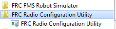
This guide will show you how to use the FRC® Radio Configuration Utility software to configure your robot’s wireless bridge for use outside of FRC events.
Prerequisites
The FRC Radio Configuration Utility requires administrator privileges to configure the network settings on your machine. The program should request the necessary privileges automatically (may require a password if run from a non-administrator account), but if you are having trouble, try running it from an administrator account.
Download the latest FRC Radio Configuration Utility Installer from the following links:
FRC Radio Configuration 22.0.1
FRC Radio Configuration 22.0.1 Israel Version
Note
The _IL version is for Israel teams and contains a version of the OM5PAC firmware with restricted channels for use in Israel.
Before you begin using the software:
Plug directly from your computer into the wireless bridge ethernet port closest to the power jack. Make sure no other devices are connected to your computer via ethernet. If powering the radio via PoE, plug an Ethernet cable from the PC into the socket side of the PoE adapter (where the roboRIO would plug in). If you experience issues configuring through the PoE adapter, you may try connecting the PC to the alternate port on the radio.
Warning
The OM5P-AN and AC use the same power plug as the D-Link DAP1522, however they are 12V radios. Wire the radio to the 12V 2A terminals on the VRM (center-pin positive).
Application Notes
By default, the Radio Configuration Utility will program the radio to enforce the 4Mbps bandwidth limit on traffic exiting the radio over the wireless interface. In the home configuration (AP mode) this is a total, not a per client limit. This means that streaming video to multiple clients is not recommended.
The Utility has been tested on Windows 7, 8 and 10. It may work on other operating systems, but has not been tested.
Programmed Configuration
The Radio Configuration Utility programs a number of configuration settings into the radio when run. These settings apply to the radio in all modes (including at events). These include:
Set a static IP of
10.TE.AM.1Set an alternate IP on the wired side of
192.168.1.1for future programmingBridge the wired ports so they may be used interchangeably
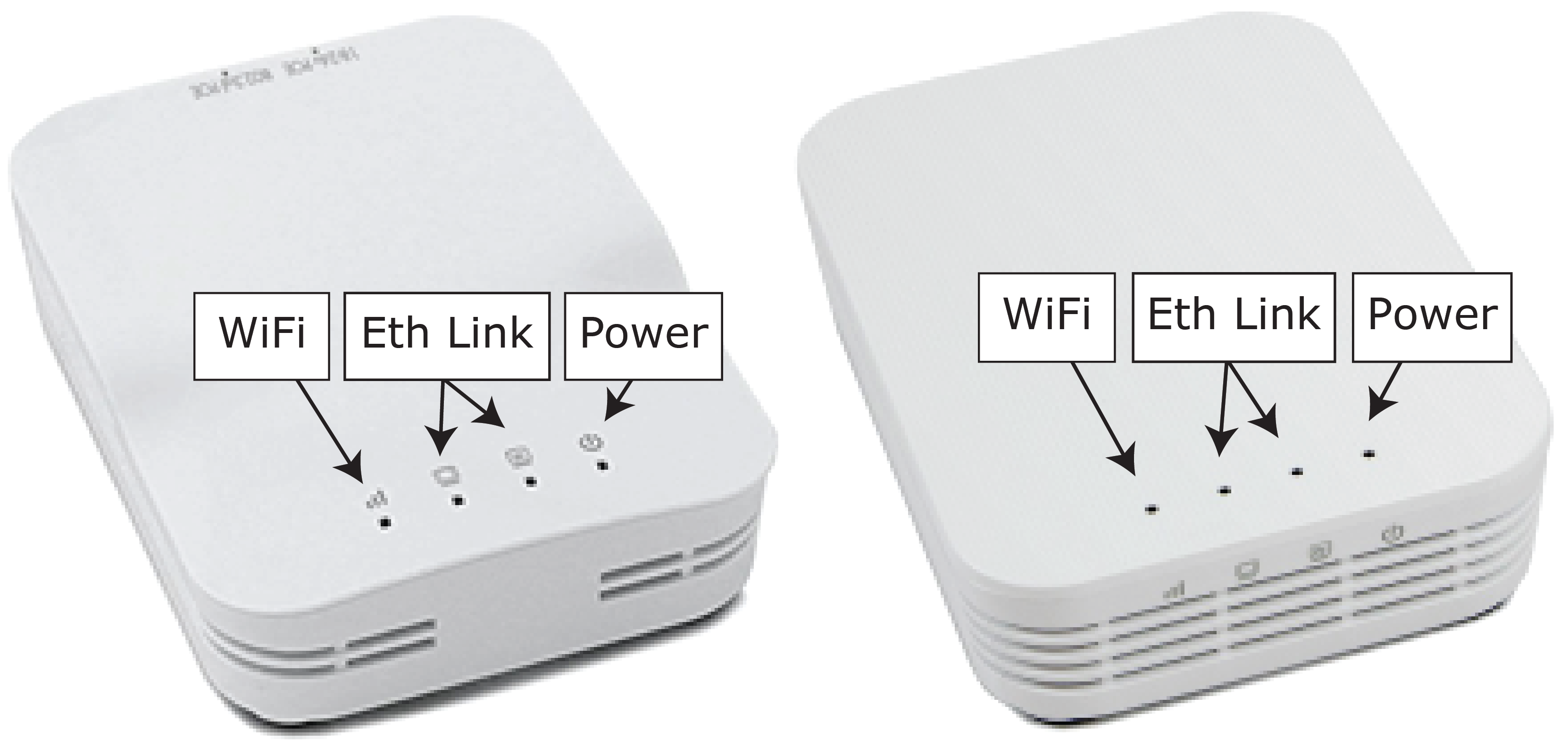
The LED configuration noted in the graphic above.
4Mb/s bandwidth limit on the outbound side of the wireless interface (may be disabled for home use)
QoS rules for internal packet prioritization (affects internal buffer and which packets to discard if bandwidth limit is reached). These rules are:
Robot Control and Status (UDP
1110,1115,1150)Robot TCP & NetworkTables (TCP
1735,1740)Bulk (All other traffic). (disabled if BW limit is disabled)
DHCP server enabled. Serves out:
10.TE.AM.11-10.TE.AM.111on the wired side10.TE.AM.138-10.TE.AM.237on the wireless sideSubnet mask of
255.255.255.0Broadcast address
10.TE.AM.255
DNS server enabled. DNS server IP and domain suffix (
.lan) are served as part of the DHCP.
At home only:
SSID may have a “Robot Name” appended to the team number to distinguish multiple networks.
Firewall option may be enabled to mimic the field firewall rules (open ports may be found in the Game Manual)
Warning
It is not possible to modify the configuration manually.
Install the Software

Double click on FRC_Radio_Configuration_VERSION.exe to launch the installer. Follow the prompts to complete the installation.
Part of the installation prompts will include installing Npcap if it is not already present. The Npcap installer contains a number of checkboxes to configure the install. You should leave the options as the defaults.
Launch the software
Use the Start menu or desktop shortcut to launch the program.
Note
If you need to locate the program, it is installed to C:\Program Files (x86)\FRC Radio Configuration Utility. For 32-bit machines the path is C:\Program Files\FRC Radio Configuration Utility
Allow the program to make changes, if prompted
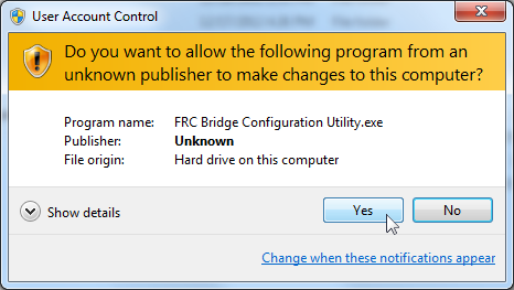
A prompt may appear about allowing the configuration utility to make changes to the computer. Click Yes if the prompt appears.
Select the network interface
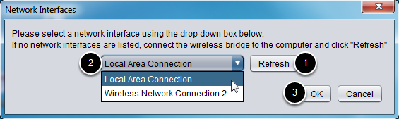
Use the pop-up window to select the which ethernet interface the configuration utility will use to communicate with the wireless bridge. On Windows machines, ethernet interfaces are typically named “Local Area Connection”. The configuration utility can not program a bridge over a wireless connection.
If no ethernet interfaces are listed, click Refresh to re-scan for available interfaces.
Select the interface you want to use from the drop-down list.
Click OK.
Open Mesh Firmware Note
For the FRC Radio Configuration Utility to program the OM5P-AN and OM5P-AC radio, the radio must be running an FRC specific build of the OpenWRT firmware.
If you do not need to update or re-load the firmware, skip the next step.
Warning
Radios used in 2019/2020/2021 do not need to be updated before configuring, the 2022 tool uses the same 2019 firmware.
Loading FRC Firmware to Open Mesh Radio
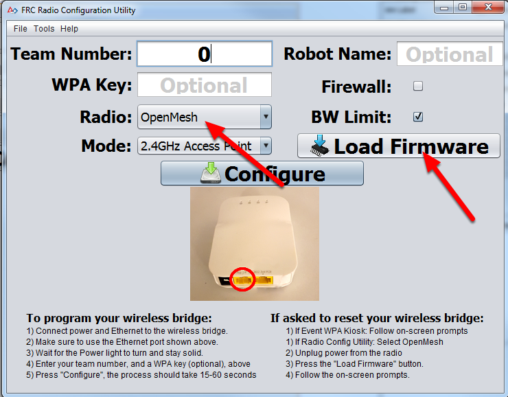
If you need to load the FRC firmware (or reset the radio), you can do so using the FRC Radio Configuration Utility.
Follow the instructions above to install the software, launch the program and select the Ethernet interface.
Make sure the Open Mesh radio is selected in the Radio dropdown.
Make sure the radio is connected to the PC via Ethernet.
Unplug the power from the radio. (If using a PoE cable, this will also be unplugging the Ethernet to the PC, this is fine)
Press the Load Firmware button
When prompted, plug in the radio power. The software should detect the radio, load the firmware and prompt you when complete.
Warning
If you see an error about NPF name, try disabling all adapters other than the one being used to program the radio. If only one adapter is found, the tool should attempt to use that one. See the steps in Disabling Network Adapters for more info.
Teams may also see this error with foreign language Operating Systems. If you experience issues loading firmware or programming on a foreign language OS, try using an English OS, such as on the KOP provided PC or setting the Locale setting to “en_us” as described on this page.
Select Radio and Operating Mode
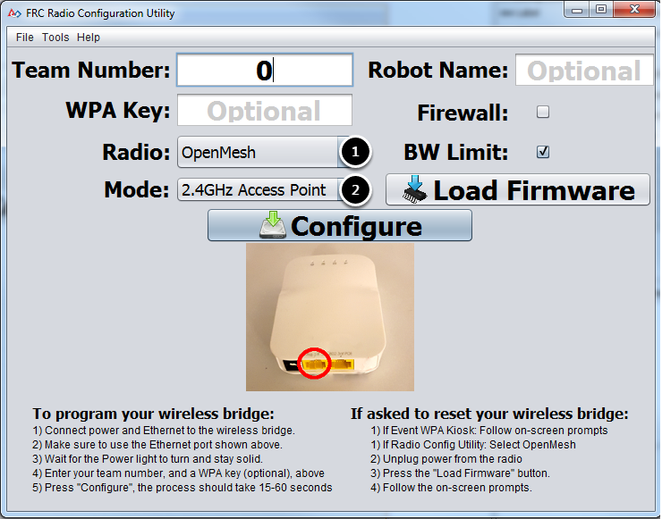
Select which radio you are configuring using the drop-down list.
Select which operating mode you want to configure. For most cases, the default selection of 2.4GHz Access Point will be sufficient. If your computers support it, the 5GHz AP mode is recommended, as 5GHz is less congested in many environments.
Select Options
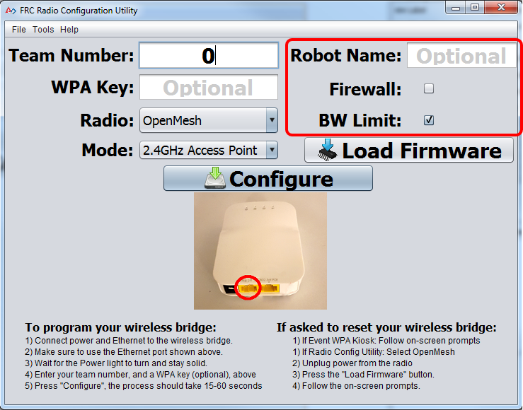
The default values of the options have been selected to match the use case of most teams, however, you may wish to customize these options to your specific scenario:
Robot Name: This is a string that gets appended to the SSID used by the radio. This allows you to have multiple networks with the same team number and still be able to distinguish them.
Firewall: If this box is checked, the radio firewall will be configured to attempt to mimic the port blocking behavior of the firewall present on the FRC field. For a list of open ports, please see the FRC Game Manual.
BW Limit: If this box is checked, the radio enforces a 4 Mbps bandwidth limit like it does when programmed at events. Note that this is a total limit, not per client, so streaming video to multiple clients simultaneously may cause undesired behavior.
Note
Firewall and BW Limit only apply to the Open Mesh radios. These options have no effect on D-Link radios.
Warning
The “Firewall” option configures the radio to emulate the field firewall. This means that you will not be able to deploy code wirelessly with this option enabled. This is useful for simulating blocked ports that may exist at competitions.
Starting the Configuration Process
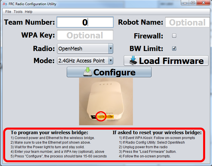
Follow the on-screen instructions for preparing your wireless bridge, entering the settings the bridge will be configured with, and starting the configuration process. These on-screen instructions update to match the bridge model and operating mode chosen.
Configuration Progress
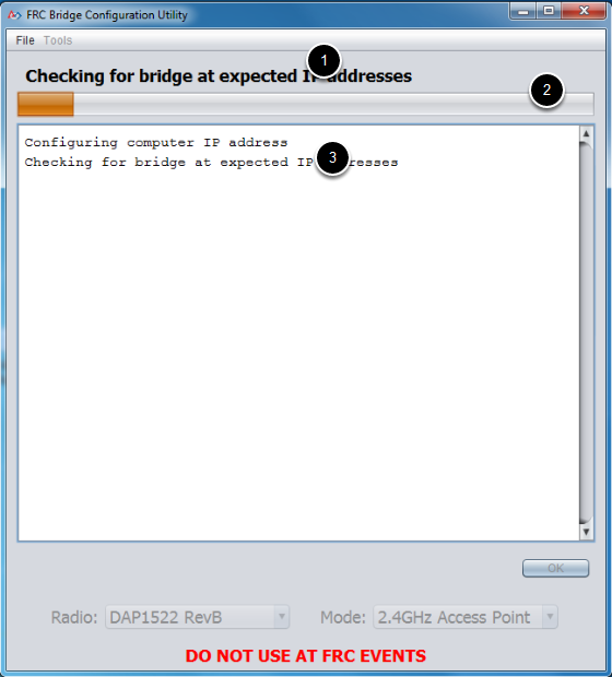
Throughout the configuration process, the window will indicate:
The step currently being executed.
The overall progress of the configuration process.
All steps executed so far.
Configuration Completed
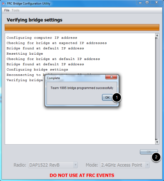
Once the configuration is complete:
Press OK on the dialog window.
Press OK on the main window to return to the settings screen.
Configuration Errors
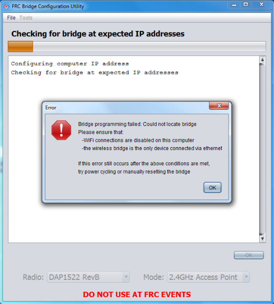
If an error occurs during the configuration process, follow the instructions in the error message to correct the problem.
Troubleshooting
Make sure you wait long enough that the power light has stayed solid for 10 seconds.
Make sure you have the correct network interface, and only one interface is listed in the drop-down.
Make sure your firewall is turned off.
Plug directly from your computer into the wireless bridge and make sure no other devices are connected to your computer via ethernet.
Ensure the ethernet is plugged into the port closest to the power jack on the wireless bridge.
If using a foreign language Operating System, try using an English OS, such as on the KOP provided PC or setting the Locale setting to “en_us” as described on this page.
If all else fails, try a different computer.
Step 4: Programming your Robot
Creating your Benchtop Test Program (LabVIEW)
Note
This document covers how to create, build and load an FRC® LabVIEW program onto a roboRIO. Before beginning, make sure that you have installed LabVIEW for FRC and the FRC Game Tools and that you have configured and imaged your roboRIO as described in the Zero-to-Robot tutorial.
Creating a Project
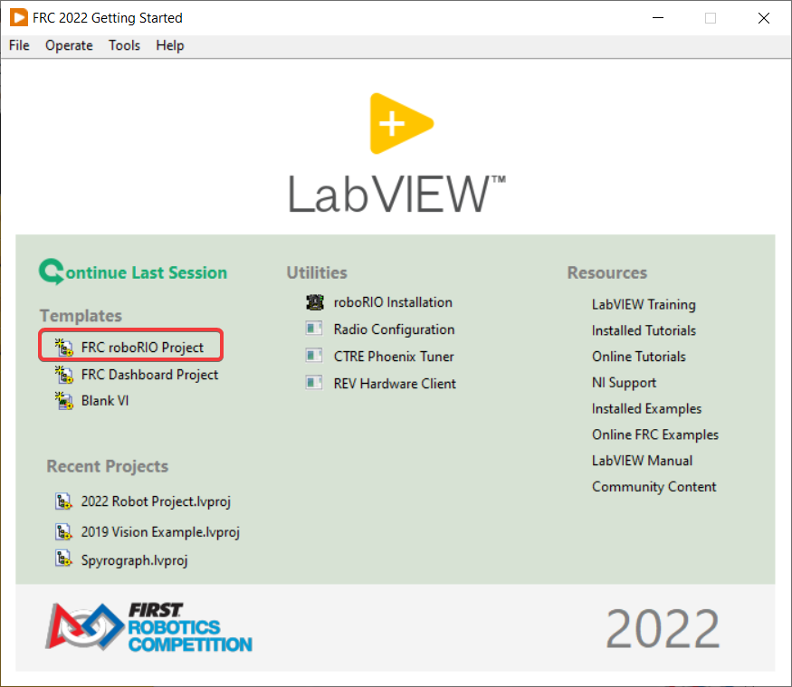
Launch LabVIEW and click the FRC roboRIO Robot Project link to display the Create New FRC Robot Project dialog box.
Configuring Project
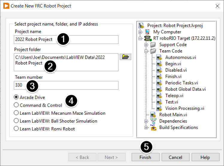
Fill in the Create New FRC Project Dialog:
Pick a name for your project
Select a folder to place the project in.
Enter your team number
Select a project type. If unsure, select Arcade Drive.
Click Finish
Running the Program
Note
Note that a program deployed in this manner will not remain on the roboRIO after a power cycle. To deploy a program to run every time the roboRIO starts follow the next step, Deploying the program.
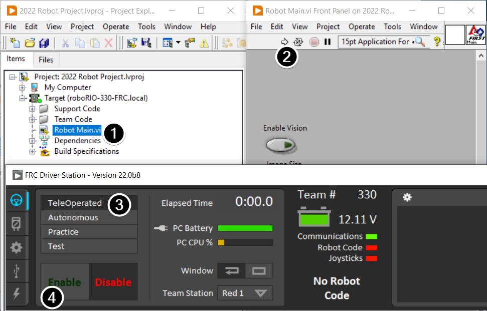
In the Project Explorer window, double-click the Robot Main.vi item to open the Robot Main VI.
Click the Run button (White Arrow on the top ribbon) of the Robot Main VI to deploy the VI to the roboRIO. LabVIEW deploys the VI, all items required by the VI, and the target settings to memory on the roboRIO. If prompted to save any VIs, click Save on all prompts.
Using the Driver Station software, put the robot in Teleop Mode. For more information on configuring and using the Driver Station software, see the FRC Driver Station Software article.
Click Enable.
Move the joysticks and observe how the robot responds.
Click the Abort button of the Robot Main VI. Notice that the VI stops. When you deploy a program with the Run button, the program runs on the roboRIO, but you can manipulate the front panel objects of the program from the host computer.
Deploying the Program
To run in the competition, you will need to deploy a program to your roboRIO. This allows the program to survive across reboots of the controller, but doesn’t allow the same debugging features (front panel, probes, highlight execution) as running from the front panel. To deploy your program:
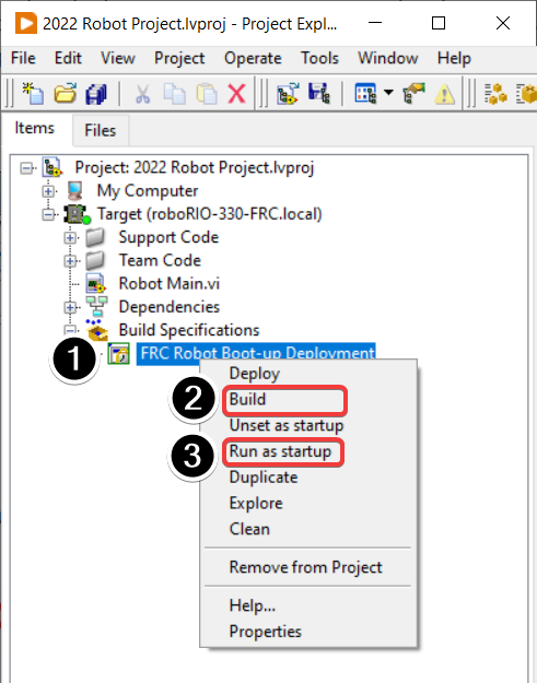
In the Project Explorer, click the + next to Build Specifications to expand it.
Right-click on FRC Robot Boot-up Deployment and select Build. Wait for the build to complete.
Right-click again on FRC Robot Boot-Up Deployment and select Run as Startup. If you receive a conflict dialog, click OK. This dialog simply indicates that there is currently a program on the roboRIO which will be terminated/replaced.
Either check the box to close the deployment window on successful completion or click the close button when the deployment completes.
The roboRIO will automatically start running the deployed code within a few seconds of the dialog closing.
Creating your Benchtop Test Program (C++/Java)
Once everything is installed, we’re ready to create a robot program. WPILib comes with several templates for robot programs. Use of these templates is highly recommended for new users; however, advanced users are free to write their own robot code from scratch. This article walks through creating a project from one of the provided examples which has some code already written to drive a basic robot.
Creating a New WPILib Project
Bring up the Visual Studio Code command palette with Ctrl+Shift+P:
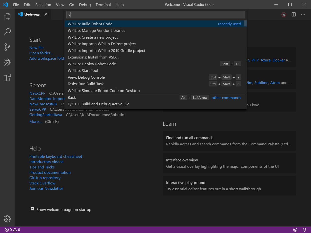
Then, type “WPILib” into the prompt. Since all WPILib commands start with “WPILib,” this will bring up the list of WPILib-specific VS Code commands:
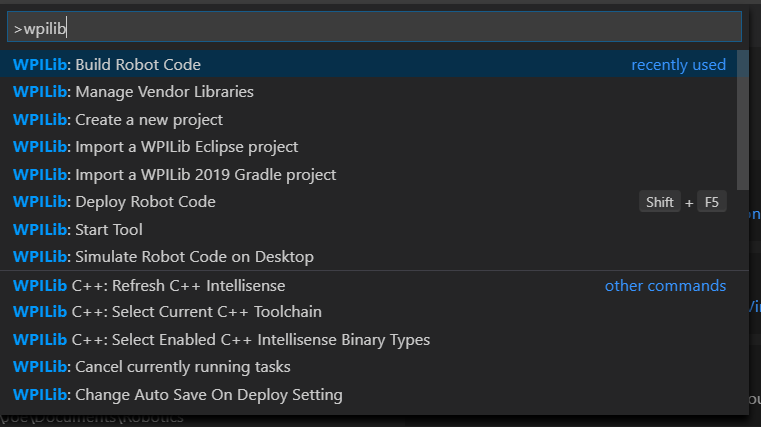
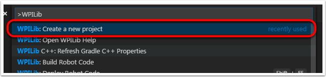
Now, select the “Create a new project” command:
This will bring up the “New Project Creator Window:”
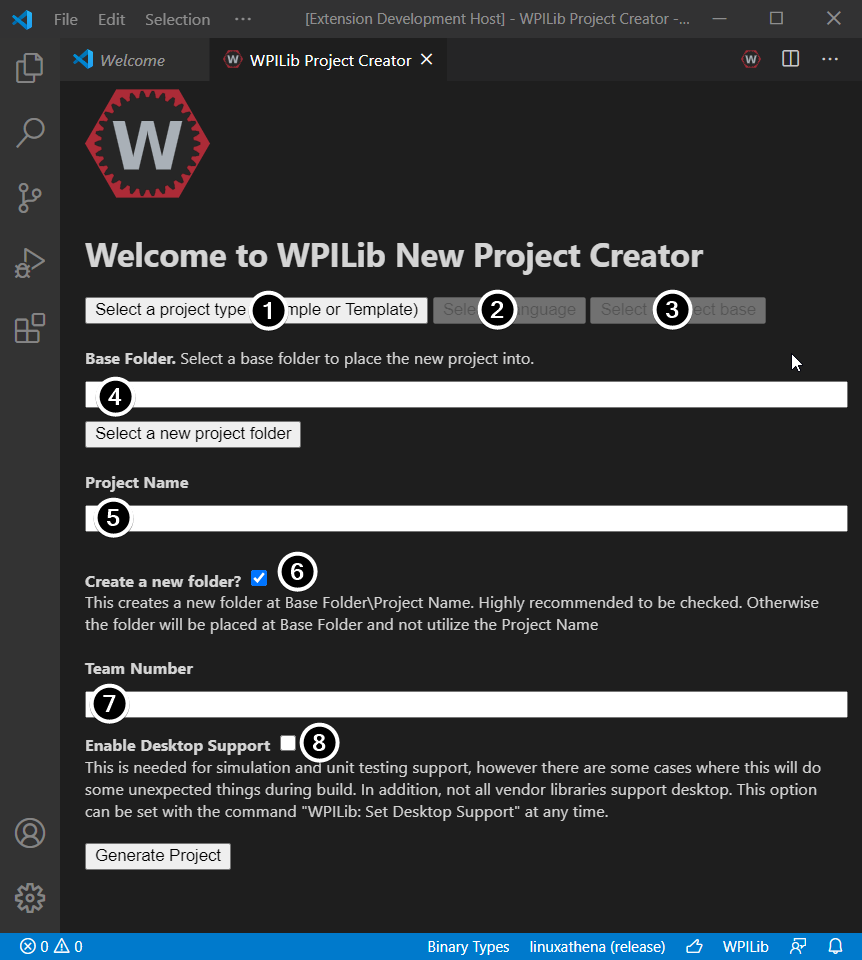
The elements of the New Project Creator Window are explained below:
Project Type: The kind of project we wish to create. For this example, select Example
Language: This is the language (C++ or Java) that will be used for this project.
Project Base: This box is used to select the base class or example to generate the project from. For this example, select Getting Started
Base Folder: This determines the folder in which the robot project will be located.
Project Name: The name of the robot project. This also specifies the name that the project folder will be given if the Create New Folder box is checked.
Create a New Folder: If this is checked, a new folder will be created to hold the project within the previously-specified folder. If it is not checked, the project will be located directly in the previously-specified folder. An error will be thrown if the folder is not empty and this is not checked. project folder will be given if the Create New Folder box is checked.
Team Number: The team number for the project, which will be used for package names within the project and to locate the robot when deploying code.
Enable Desktop Support: Enables unit test and simulation. While WPILib supports this, third party software libraries may not. If libraries do not support desktop, then your code may not compile or may crash. It should be left unchecked unless unit testing or simulation is needed and all libraries support it. For this example, do not check this box.
Once all the above have been configured, click “Generate Project” and the robot project will be created.
Note
Any errors in project generation will appear in the bottom right-hand corner of the screen.
Opening The New Project
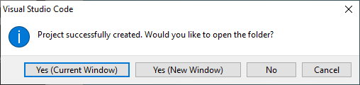
After successfully creating your project, VS Code will give the option of opening the project as shown above. We can choose to do that now or later by typing Ctrl+K then Ctrl+O (or just Command+O on macOS) and select the folder where we saved our project.
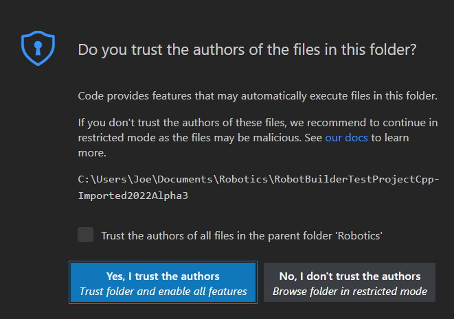
Click Yes I trust the authors.
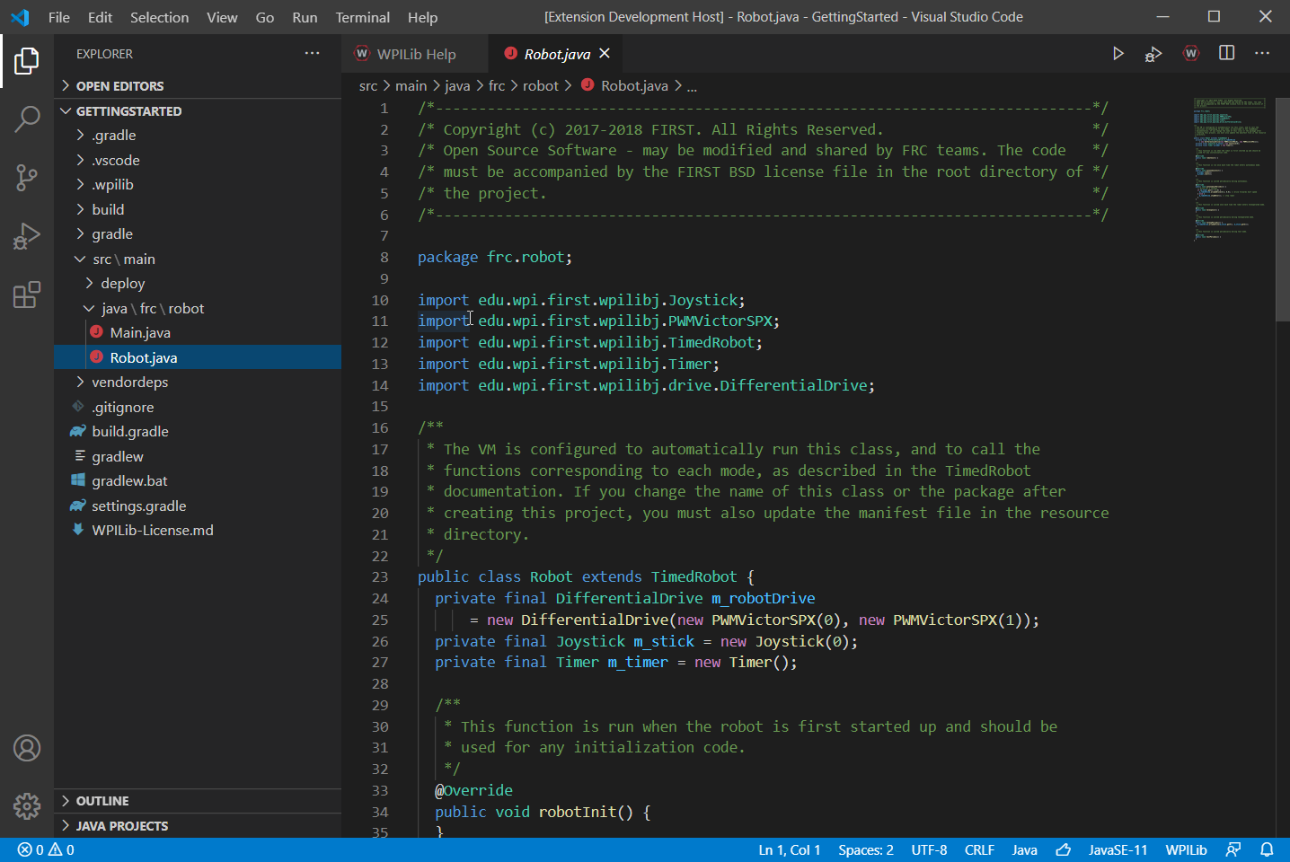
Once opened we will see the project hierarchy on the left. Double clicking on the file will open that file in the editor.
C++ Configurations (C++ Only)
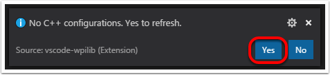
For C++ projects, there is one more step to set up IntelliSense. Whenever we open a project, we should get a pop-up in the bottom right corner asking to refresh C++ configurations. Click “Yes” to set up IntelliSense.
Imports/Includes
 7import edu.wpi.first.wpilibj.Joystick;
 8import edu.wpi.first.wpilibj.TimedRobot;
 9import edu.wpi.first.wpilibj.Timer;
10import edu.wpi.first.wpilibj.drive.DifferentialDrive;
11import edu.wpi.first.wpilibj.motorcontrol.PWMSparkMax;
5#include <frc/Joystick.h>
6#include <frc/TimedRobot.h>
7#include <frc/Timer.h>
8#include <frc/drive/DifferentialDrive.h>
9#include <frc/motorcontrol/PWMSparkMax.h>
Our code needs to reference the components of WPILib that are used. In C++ this is accomplished using #include statements; in Java it is done with import statements. The program references classes for Joystick (for driving), PWMSparkMax (for controlling motors), TimedRobot (the base class used for the example), Timer (used for autonomous), DifferentialDrive (for connecting the joystick control to the motors), and LiveWindow (C++ only).
Defining the variables for our sample robot
19public class Robot extends TimedRobot {
20  private final PWMSparkMax m_leftDrive = new PWMSparkMax(0);
21  private final PWMSparkMax m_rightDrive = new PWMSparkMax(1);
22  private final DifferentialDrive m_robotDrive = new DifferentialDrive(m_leftDrive, m_rightDrive);
23  private final Joystick m_stick = new Joystick(0);
24  private final Timer m_timer = new Timer();
12 public:
13  Robot() {
14    m_right.SetInverted(true);
15    m_robotDrive.SetExpiration(100_ms);
16    // We need to invert one side of the drivetrain so that positive voltages
17    // result in both sides moving forward. Depending on how your robot's
18    // gearbox is constructed, you might have to invert the left side instead.
19    m_timer.Start();
20  }
49 private:
50  // Robot drive system
51  frc::PWMSparkMax m_left{0};
52  frc::PWMSparkMax m_right{1};
53  frc::DifferentialDrive m_robotDrive{m_left, m_right};
54
55  frc::Joystick m_stick{0};
56  frc::Timer m_timer;
57};
The sample robot in our examples will have a joystick on USB port 0 for arcade drive and two motors on PWM ports 0 and 1. Here we create objects of type DifferentialDrive (m_robotDrive), Joystick (m_stick) and Timer (m_timer). This section of the code does three things:
Defines the variables as members of our Robot class.
Initializes the variables.
Note
The variable initializations for C++ are in the private section at the bottom of the program. This means they are private to the class (Robot). The C++ code also sets the Motor Safety expiration to 0.1 seconds (the drive will shut off if we don’t give it a command every .1 seconds) and starts the Timer used for autonomous.
Robot Initialization
@Override
public void robotInit() {}
void RobotInit() {}
The RobotInit method is run when the robot program is starting up, but after the constructor. The RobotInit for our sample program doesn’t do anything. If we wanted to run something here we could provide the code above to override the default).
Simple Autonomous Example
38  /** This function is run once each time the robot enters autonomous mode. */
39  @Override
40  public void autonomousInit() {
41    m_timer.reset();
42    m_timer.start();
43  }
44
45  /** This function is called periodically during autonomous. */
46  @Override
47  public void autonomousPeriodic() {
48    // Drive for 2 seconds
49    if (m_timer.get() < 2.0) {
50      m_robotDrive.arcadeDrive(0.5, 0.0); // drive forwards half speed
51    } else {
52      m_robotDrive.stopMotor(); // stop robot
53    }
54  }
22  void AutonomousInit() override {
23    m_timer.Reset();
24    m_timer.Start();
25  }
26
27  void AutonomousPeriodic() override {
28    // Drive for 2 seconds
29    if (m_timer.Get() < 2_s) {
30      // Drive forwards half speed
31      m_robotDrive.ArcadeDrive(0.5, 0.0);
32    } else {
33      // Stop robot
34      m_robotDrive.ArcadeDrive(0.0, 0.0);
35    }
36  }
The AutonomousInit method is run once each time the robot transitions to autonomous from another mode. In this program, we reset the Timer and then start it in this method.
AutonomousPeriodic is run once every period while the robot is in autonomous mode. In the TimedRobot class the period is a fixed time, which defaults to 20ms. In this example, the periodic code checks if the timer is less than 2 seconds and if so, drives forward at half speed using the ArcadeDrive method of the DifferentialDrive class. If more than 2 seconds has elapsed, the code stops the robot drive.
Joystick Control for teleoperation
56  /** This function is called once each time the robot enters teleoperated mode. */
57  @Override
58  public void teleopInit() {}
59
60  /** This function is called periodically during teleoperated mode. */
61  @Override
62  public void teleopPeriodic() {
63    m_robotDrive.arcadeDrive(m_stick.getY(), m_stick.getX());
64  }
38  void TeleopInit() override {}
39
40  void TeleopPeriodic() override {
41    // Drive with arcade style (use right stick)
42    m_robotDrive.ArcadeDrive(-m_stick.GetY(), m_stick.GetX());
43  }
Like in Autonomous, the Teleop mode has a TeleopInit and TeleopPeriodic function. In this example we don’t have anything to do in TeleopInit, it is provided for illustration purposes only. In TeleopPeriodic, the code uses the ArcadeDrive method to map the Y-axis of the Joystick to forward/back motion of the drive motors and the X-axis to turning motion.
Test Mode
66  /** This function is called once each time the robot enters test mode. */
67  @Override
68  public void testInit() {}
69
70  /** This function is called periodically during test mode. */
71  @Override
72  public void testPeriodic() {}
73}
45  void TestInit() override {}
46
47  void TestPeriodic() override {}
Test Mode is used for testing robot functionality. Similar to TeleopInit, the TestInit and TestPeriodic methods are provided here for illustrative purposes only.
Running your Benchtop Test Program
Overview
You should create and download a Benchtop Test Program as described for your programming language:
Tethered Operation
Running your benchtop testing program while tethered to the Driver Station via ethernet or USB cable will confirm the the program was successfully deployed and that the driver station and roboRIO are properly configured.
The roboRIO should be powered on and connected to the PC over Ethernet or USB.
Starting the FRC Driver Station
The FRC® Driver Station can be launched by double-clicking the icon on the Desktop or by selecting Start->All Programs->FRC Driver Station.
Setting Up the Driver Station
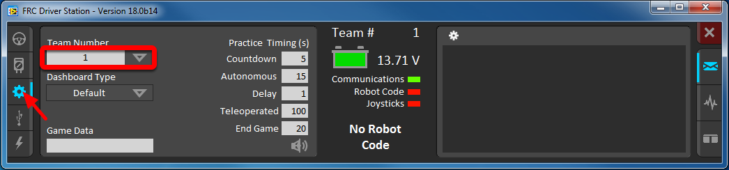
The DS must be set to your team number in order to connect to your robot. In order to do this click the Setup tab then enter your team number in the team number box. Press return or click outside the box for the setting to take effect.
PCs will typically have the correct network settings for the DS to connect to the robot already, but if not, make sure your Network adapter is set to DHCP.
Confirm Connectivity
Tethered
Wireless
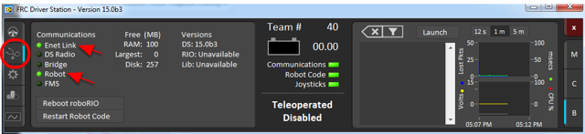
Using the Driver Station software, click Diagnostics and confirm that the Enet Link (or Robot Radio led, if operating wirelessly) and Robot leds are green.
Operate the Robot
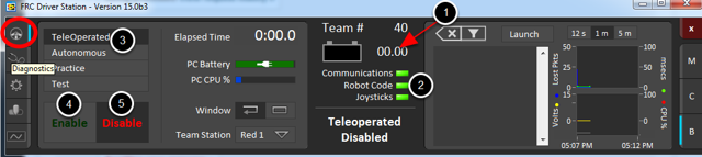
Click the Operation Tab
Confirm that battery voltage is displayed
Communications, Robot Code, and Joysticks indicators are green.
Put the robot in Teleop Mode
Click Enable. Move the joysticks and observe how the robot responds.
Click Disable
Wireless Operation
Before attempting wireless operation, tethered operation should have been confirmed as described in Tethered Operation. Running your benchtop testing program while connected to the Driver Station via WiFi will confirm that the access point is properly configured.
Configuring the Access Point
See the article Programming your radio for details on configuring the robot radio for use as an access point.
After configuring the access point, connect the driver station wirelessly to the robot. The SSID will be your team number (as entered in the Bridge Configuration Utility). If you set a key when using the Bridge Configuration Utility you will need to enter it to connect to the network. Make sure the computer network adapter is set to DHCP (“Obtain an IP address automatically”).
You can now confirm wireless operation using the same steps in Confirm Connectivity and Operate the Robot above.
Hardware Component Overview
The goal of this document is to provide a brief overview of the hardware components that make up the FRC® Control System. Each component will contain a brief description of the component function and a link to more documentation.
Note
For complete wiring instructions/diagrams, please see the Wiring the FRC Control System document.
Overview of Control System

Diagram courtesy of FRC® Team 3161 and Stefen Acepcion.

Diagram courtesy of FRC® Team 3161 and Stefen Acepcion.
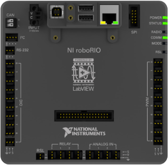
NI roboRIO
The NI-roboRIO is the main robot controller used for FRC. The roboRIO serves as the “brain” for the robot running team-generated code that commands all of the other hardware.
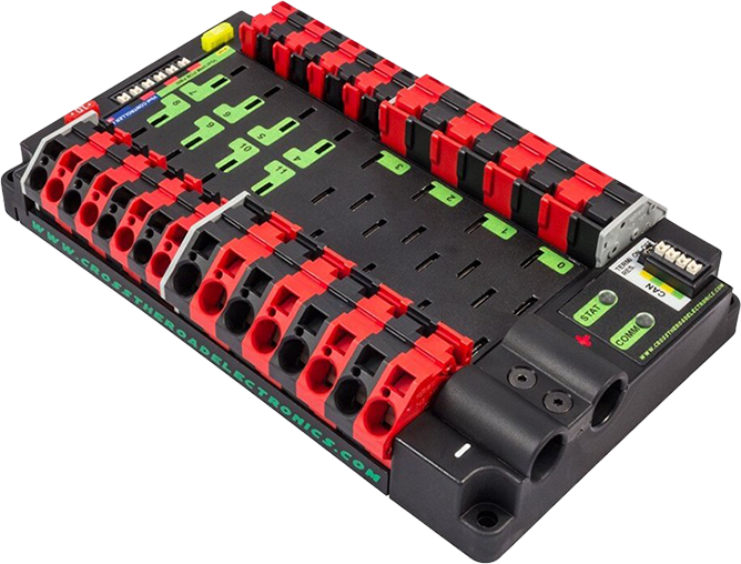
CTRE Power Distribution Panel
The CTRE Power Distribution Panel (PDP) is designed to distribute power from a 12VDC battery to various robot components through auto-resetting circuit breakers and a small number of special function fused connections. The PDP provides 8 output pairs rated for 40A continuous current and 8 pairs rated for 30A continuous current. The PDP provides dedicated 12V connectors for the roboRIO, as well as connectors for the Voltage Regulator Module and Pneumatics Control Module. It also includes a CAN interface for logging current, temperature, and battery voltage. For more detailed information, see the PDP User Manual.
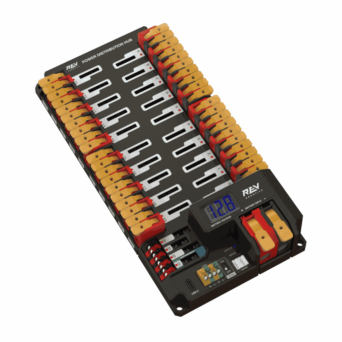
REV Power Distribution Hub
The REV Power Distribution Hub (PDH) is designed to distribute power from a 12VDC battery to various robot components. The PDH features 20 high-current (40A max) channels, 3 low-current (15A max), and 1 switchable low-current channel. The Power Distribution Hub features toolless latching WAGO terminals, an LED voltage display, and the ability to connect over CAN or USB-C to the REV Hardware Client for real-time telemetry.
CTRE Voltage Regulator Module
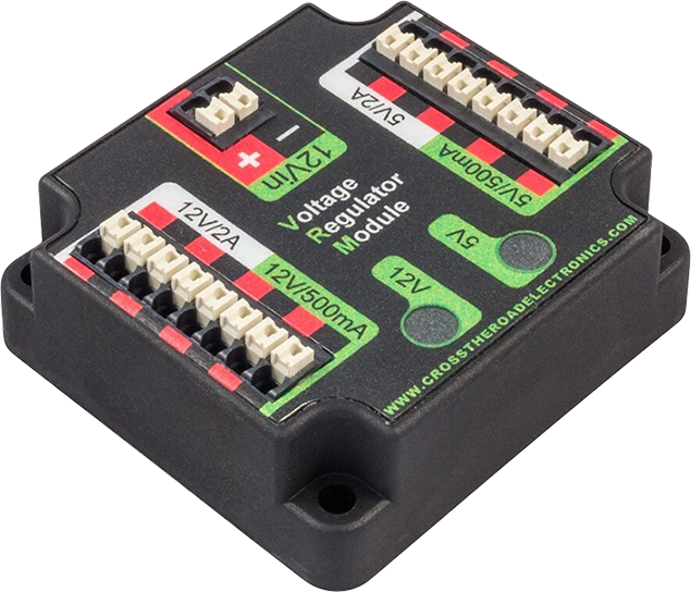
The CTRE Voltage Regulator Module (VRM) is an independent module that is powered by 12 volts. The device is wired to a dedicated connector on the PDP. The module has multiple regulated 12V and 5V outputs. The purpose of the VRM is to provide regulated power for the robot radio, custom circuits, and IP vision cameras. For more information, see the VRM User Manual.
REV Radio Power Module
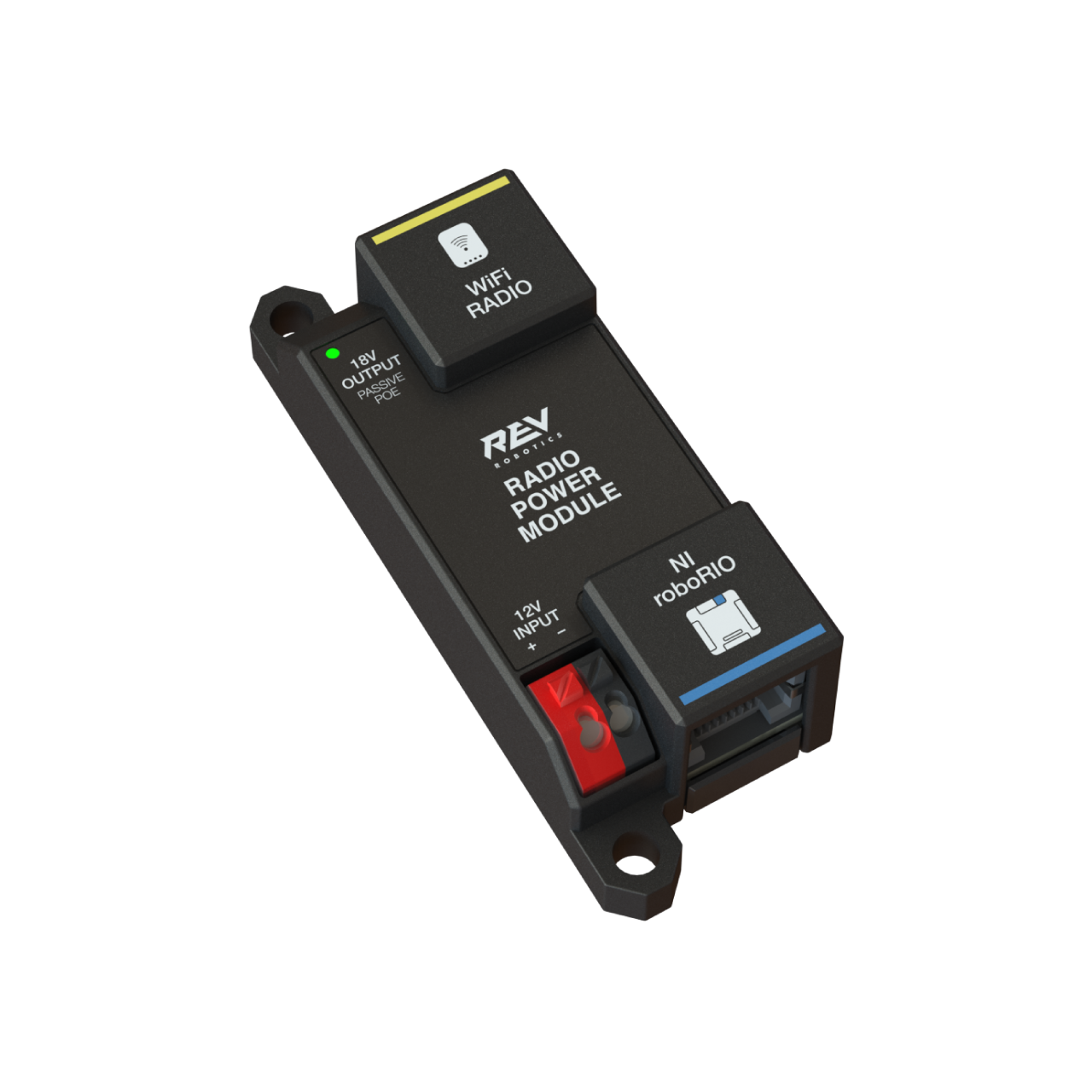
The REV Radio Power Module is designed to keep one of the most critical system components, the OpenMesh WiFi radio, powered in the toughest moments of the competition. The Radio Power Module eliminates the need for powering the radio through a traditional barrel power jack. Utilizing 18V Passive POE with two socketed RJ45 connectors, the Radio Power Module passes signal between the radio and roboRIO while providing power directly to the radio. After connecting the radio and roboRIO, easily add power to the Radio Power Module by wiring it to the low-current channels on the Power Distribution Hub utilizing the color coded push button WAGO terminals.
OpenMesh OM5P-AN or OM5P-AC Radio

Either the OpenMesh OM5P-AN or OpenMesh OM5P-AC wireless radio is used as the robot radio to provide wireless communication functionality to the robot. The device can be configured as an Access Point for direct connection of a laptop for use at home. It can also be configured as a bridge for use on the field. The robot radio should be powered by one of the 12V/2A outputs on the VRM and connected to the roboRIO controller over Ethernet. For more information, see Programming your Radio.
The OM5P-AN is no longer available for purchase. The OM5P-AC is slightly heavier, has more cooling grates, and has a rough surface texture compared to the OM5P-AN.
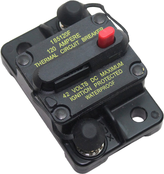
120A Circuit Breaker
The 120A Main Circuit Breaker serves two roles on the robot: the main robot power switch and a protection device for downstream robot wiring and components. The 120A circuit breaker is wired to the positive terminals of the robot battery and Power Distribution boards. For more information, please see the Cooper Bussmann 18X Series Datasheet (PN: 185120F)
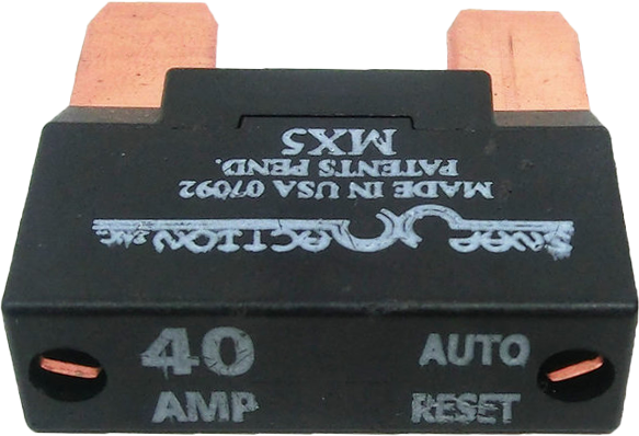
Snap Action Circuit Breakers
The Snap Action circuit breakers, MX5 series and VB3 Series, are used with the Power Distribution Panel to limit current to branch circuits. The ratings on these circuit breakers are for continuous current, temporary peak values can be considerably higher.
Robot Battery

The power supply for an FRC robot is a single 12V 18Ah Sealed Lead Acid (SLA) battery, capable of meeting the high current demands of an FRC robot. For more information, see the Robot Battery page.
Note
Multiple battery part numbers may be legal, consult the FRC Manual for a complete list.
Robot Signal Light
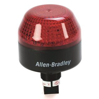
The Robot Signal Light (RSL) is required to be the Allen-Bradley 855PB-B12ME522. It is directly controlled by the roboRIO and will flash when enabled and stay solid while disabled.
CTRE Pneumatics Control Module
The CTRE Pneumatics Control Module (PCM) contains all of the inputs and outputs required to operate 12V or 24V pneumatic solenoids and the on board compressor. The PCM contains an input for the pressure sensor and will control the compressor automatically when the robot is enabled and a solenoid has been created in the code. For more information see the PCM User Manual.
REV Pneumatic Hub
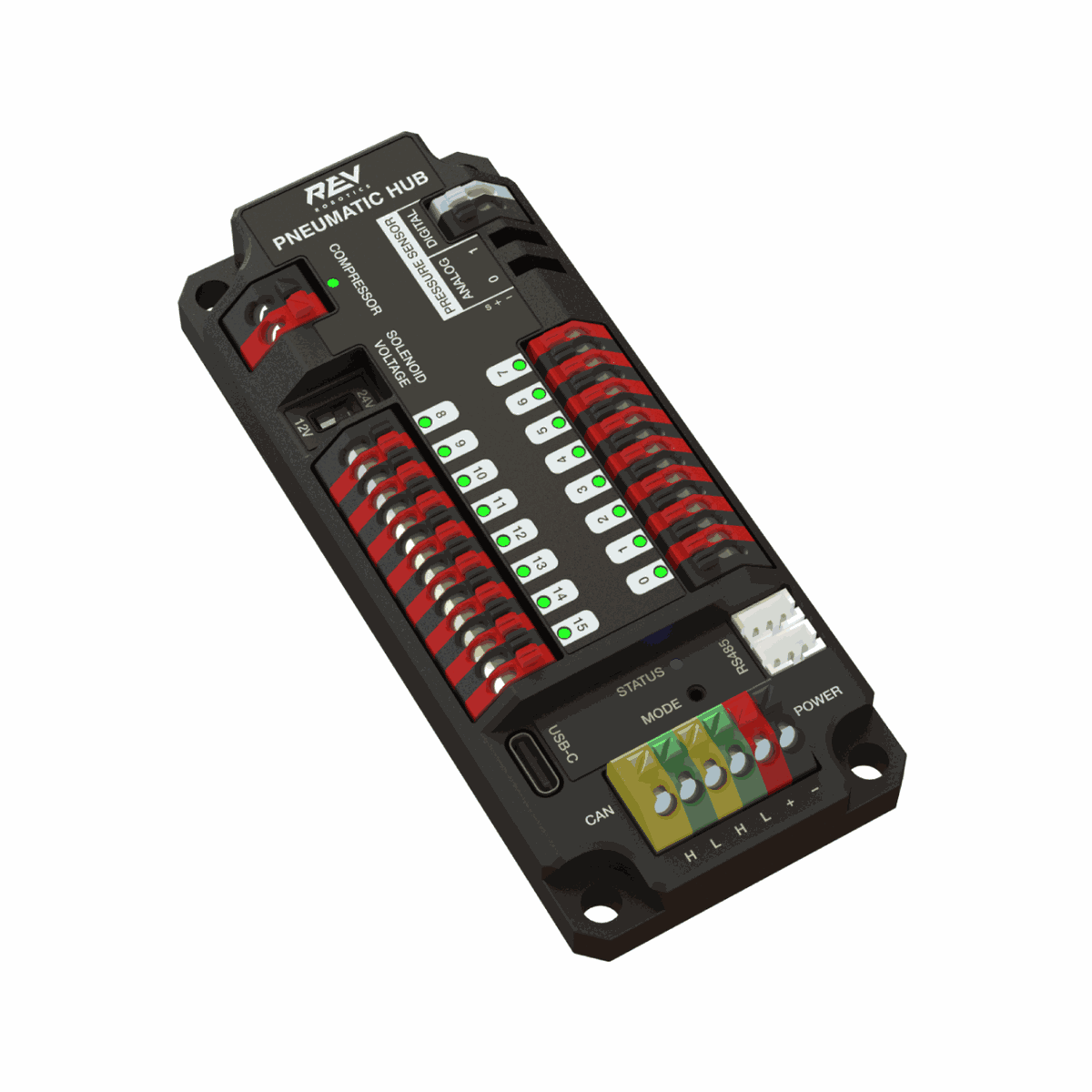
The REV Pneumatic Hub is a standalone module that is capable of switching both 12V and 24V pneumatic solenoid valves. The Pneumatic Hub features 16 solenoid channels which allow for up to 16 single-acting solenoids, 8 double-acting solenoids, or a combination of the two types. The user selectable output voltage is fully regulated, allowing even 12V solenoids to stay active when the robot battery drops as low as 4.75V.
Digital and analog pressure sensor ports are built into the device, increasing the flexibility and feedback functionality of the pneumatic system. The USB-C connection on the Hub works with the REV Hardware Client, allowing users to test pneumatic systems without a need for an additional robot controller.
Motor Controllers
There are a variety of different motor controllers which work with the FRC Control System and are approved for use. These devices are used to provide variable voltage control of the brushed and brushless DC motors used in FRC. They are listed here in order of usage.
Note
3rd Party CAN control is not supported from WPILib. See this section on Third-Party CAN Devices for more information.
Talon SRX
The Talon SRX Motor Controller is a “smart motor controller” from Cross The Road Electronics/VEX Robotics. The Talon SRX can be controlled over the CAN bus or PWM interface. When using the CAN bus control, this device can take inputs from limit switches and potentiometers, encoders, or similar sensors in order to perform advanced control. For more information see the Talon SRX User’s Guide.
Victor SPX
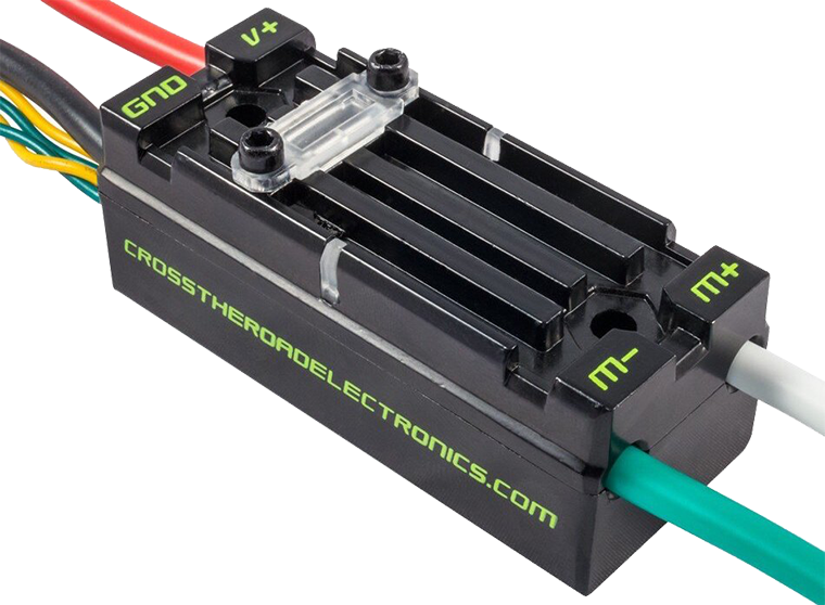
The Victor SPX Motor Controller is a CAN or PWM controlled motor controller from Cross The Road Electronics/VEX Robotics. The device is connectorized to allow easy connection to the roboRIO PWM connectors or a CAN bus. The case is sealed to prevent debris from entering the controller. For more information, see the Victor SPX User Guide.
SPARK MAX Motor Controller
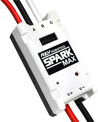
The SPARK MAX Motor Controller is an advanced brushed and brushless DC motor controller from REV Robotics. When using CAN bus or USB control, the SPARK MAX uses input from limit switches, encoders, and other sensors, including the integrated encoder of the REV NEO Brushless Motor, to perform advanced control modes. The SPARK MAX can be controlled over PWM, CAN or USB (for configuration/testing only). For more information, see the SPARK MAX User’s Manual.
TalonFX Motor Controller
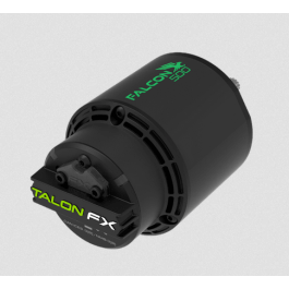
The TalonFX Motor Controller is integrated into the Falcon 500 brushless motor. It features an integrated encoder and all of the smart features of the Talon SRX and more! For more information see the Falcon 500 User Guide.
SPARK Motor Controller

Warning
While this motor controller is still legal for FRC use, the manufacturer has discontinued this product.
The SPARK Motor Controller from REV Robotics is an inexpensive brushed DC motor controller. The SPARK is controlled using the PWM interface. Limit switches may be wired directly to the SPARK to limit motor travel in one or both directions. For more information, see the SPARK User’s Manaul.
Victor SP
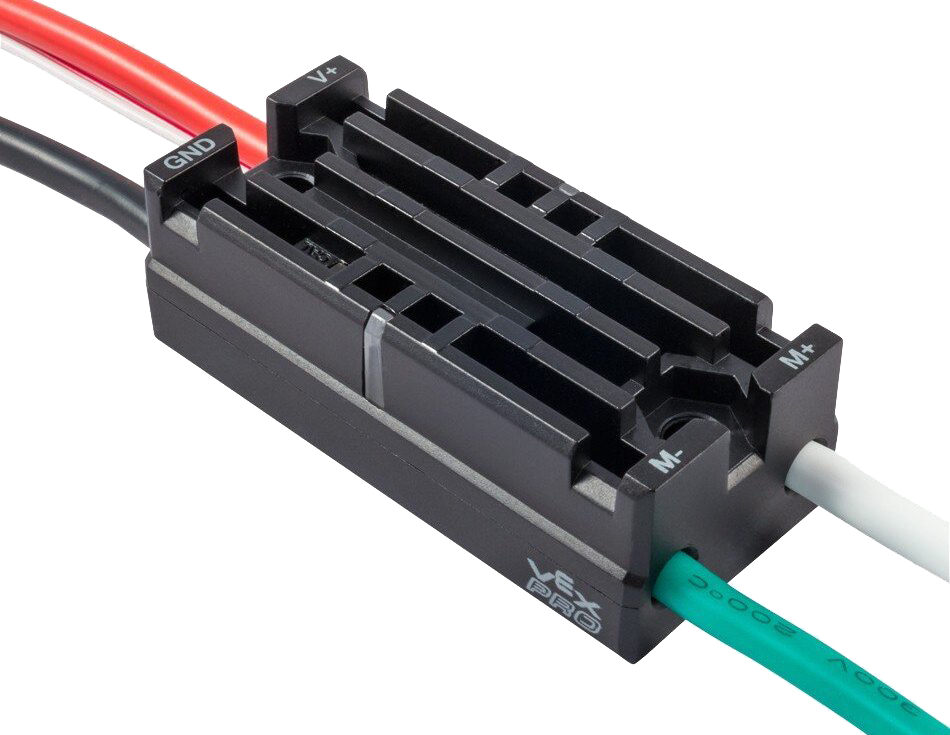
Warning
While this motor controller is still legal for FRC use, the manufacturer has discontinued this product.
The Victor SP Motor Controller is a PWM motor controller from Cross The Road Electronics/VEX Robotics. The Victor SP has an electrically isolated metal housing for heat dissipation, making the use of the fan optional. The case is sealed to prevent debris from entering the controller. The controller is approximately half the size of previous models.
Talon Motor Controller
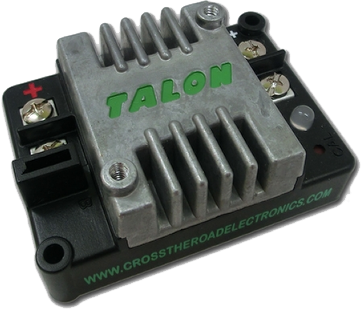
Warning
While this motor controller is still legal for FRC use, the manufacturer has discontinued this product.
The Talon Motor Controller from Cross the Road Electronics is a PWM controlled brushed DC motor controller with passive cooling.
Victor 888 Motor Controller / Victor 884 Motor Controller
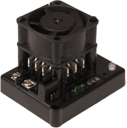
Warning
While this motor controller is still legal for FRC use, the manufacturer has discontinued this product.
The Victor 884 and Victor 888 motor controllers from VEX Robotics are variable speed PWM motor controllers for use in FRC. The Victor 888 replaces the Victor 884, which is also usable in FRC.
Jaguar Motor Controller
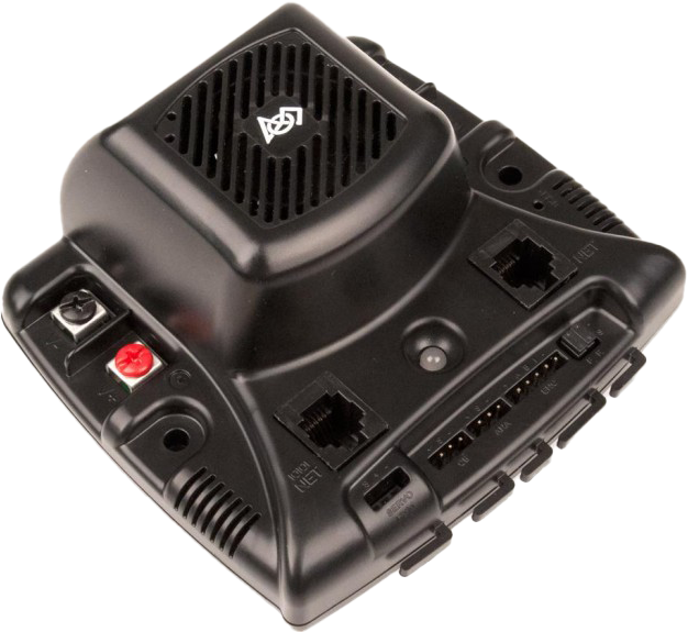
Warning
While this motor controller is still legal for FRC use, the manufacturer has discontinued this product.
The Jaguar Motor Controller from VEX Robotics (formerly made by Luminary Micro and Texas Instruments) is a variable speed motor controller for use in FRC. For FRC, the Jaguar may only be controlled using the PWM interface.
DMC-60 and DMC-60C Motor Controller
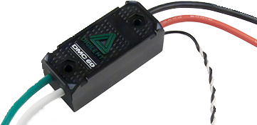
Warning
While this motor controller is still legal for FRC use, the manufacturer has discontinued this product.
The DMC-60 is a PWM motor controller from Digilent. The DMC-60 features integrated thermal sensing and protection including current-foldback to prevent overheating and damage, and four multi-color LEDs to indicate speed, direction, and status for easier debugging. For more information, see the DMC-60 reference manual
The DMC-60C adds CAN smart controller capabilities to the DMC-60 controller. Due to the manufacturer discontinuing this product, the DMC-60C is only usable with PWM. For more information see the DMC-60C Product Page
Venom Motor Controller
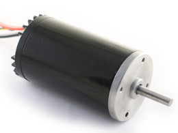
The Venom Motor Controller from Playing With Fusion is integrated into a motor based on the original CIM. Speed, current, temperature, and position are all measured onboard, enabling advanced control modes without complicated sensing and wiring schemes.
Nidec Dynamo BLDC Motor with Controller
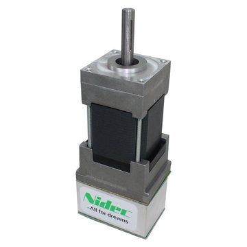
The Nidec Dynamo BLDC Motor with Controller is the first brushless motor and controller legal in FRC. This motor’s controller is integrated into the back of the motor. The motor data sheet provides more device specifics.
SD540B and SD540C Motor Controllers
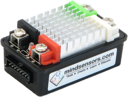
The SD540B and SD540C Motor Controllers from Mindsensors are controlled using PWM. CAN control is no longer available for the SD540C due to lack of manufacturer support. Limit switches may be wired directly to the SD540 to limit motor travel in one or both directions. For more information see the Mindsensors FRC page
Spike H-Bridge Relay
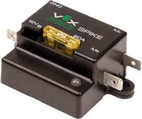
Warning
While this relay is still legal for FRC use, the manufacturer has discontinued this product.
The Spike H-Bridge Relay from VEX Robotics is a device used for controlling power to motors or other custom robot electronics. When connected to a motor, the Spike provides On/Off control in both the forward and reverse directions. The Spike outputs are independently controlled so it can also be used to provide power to up to 2 custom electronic circuits. The Spike H-Bridge Relay should be connected to a relay output of the roboRIO and powered from the Power Distribution Panel. For more information, see the Spike User’s Guide.
Servo Power Module
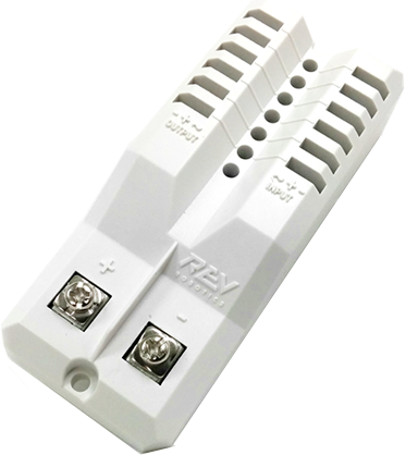
The Servo Power Module from Rev Robotics is capable of expanding the power available to servos beyond what the roboRIO integrated power supply is capable of. The Servo Power Module provides up to 90W of 6V power across 6 channels. All control signals are passed through directly from the roboRIO. For more information, see the Servo Power Module webpage.
Axis M1013/M1011/206 Ethernet Camera
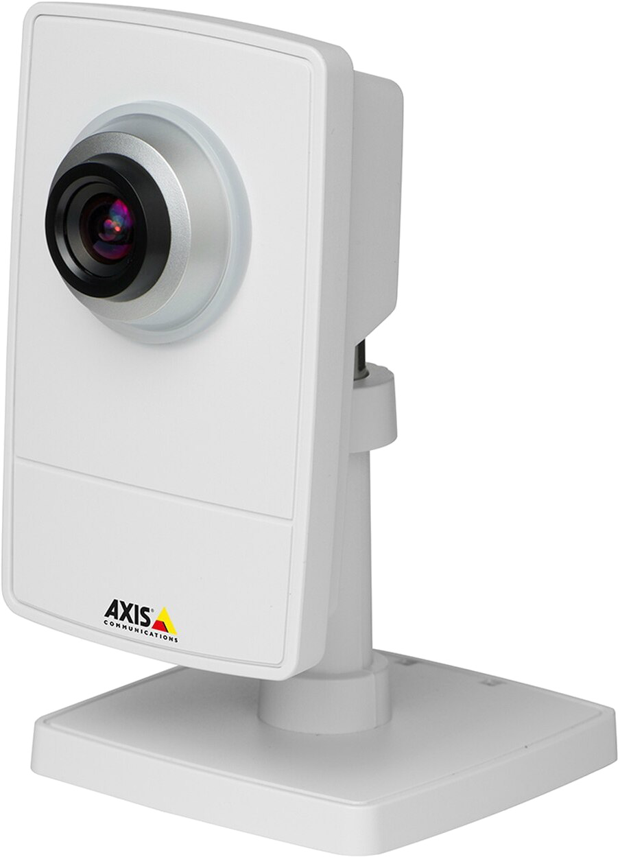
Warning
While this camera is legal for FRC use, the manufacturer has discontinued support.
The Axis M1013, M1011 and Axis 206 Ethernet cameras are used for capturing images for vision processing and/or sending video back to the Driver Station laptop. The camera should be wired to a 5V power output on the Voltage Regulator Module and an open ethernet port on the robot radio. For more information, see Configuring an Axis Camera and the Axis 206, Axis M1011, Axis M1013 pages.
Microsoft Lifecam HD3000
The Microsoft Lifecam HD3000 is a USB webcam that can be plugged directly into the roboRIO. The camera is capable of capturing up to 1280x720 video at 30 FPS. For more information about the camera, see the Microsoft product page. For more information about using the camera with the roboRIO, see the Vision Processing section of this documentation.
Image Credits
Image of roboRIO courtesy of National Instruments. Image of DMC-60 courtesy of Digilent. Image of SD540 courtesy of Mindsensors. Images of Jaguar Motor Controller, Talon SRX, Talon FX, Victor 888, Victor SP, Victor SPX, and Spike H-Bridge Relay courtesy of VEX Robotics, Inc. Image of SPARK MAX, Power Distribution Hub, Radio Power Module, and Pneumatic Hub courtesy of REV Robotics. Lifecam, PDP, PCM, SPARK, and VRM photos courtesy of FIRST®. All other photos courtesy of AndyMark Inc.
Software Component Overview
The FRC® software consists of a wide variety of mandatory and optional components. These elements are designed to assist you in the design, development, and debugging of your robot code as well as assist with control robot operation and to provide feedback when troubleshooting. For each software component this document will provide a brief overview of its purpose, a link to the package download, if appropriate, and a link to further documentation where available.
Operating System Compatibility
The primary supported OS for FRC components is Windows. All required FRC software components have been tested on Windows 10. NI Tools do not support Windows 7 or 8.1.
Warning
Support for Windows 7, 8.1, and 32 bit operating systems for all tools will be removed for the 2023 season.
Many of the tools for C++/Java programming are also supported and tested on macOS and Linux. Teams programming in C++/Java should be able to develop using these systems, using a Windows system for the Windows-only operations such as the Driver Station, Radio Configuration Utility, and roboRIO Imaging Tool.
Important
The minimum supported macOS version is Mojave (10.14.x).
LabVIEW FRC (Windows Only)
LabVIEW FRC, based on a recent version of LabVIEW Professional, is one of the three officially supported languages for programming an FRC robot. LabVIEW is a graphical, dataflow-driven language. LabVIEW programs consist of a collection of icons, called VIs, wired together with wires which pass data between the VIs. The LabVIEW FRC installer is distributed on a DVD found in the Kickoff Kit of Parts and is also available for download. A guide to getting started with the LabVIEW FRC software, including installation instructions can be found here.
Visual Studio Code
Visual Studio Code is the supported development environment for C++ and Java (the other two supported languages). Both are object-oriented text based programming languages. A guide to getting started with C++ or Java for FRC, including the installation and configuration of Visual Studio Code can be found here.
FRC Driver Station Powered by NI LabVIEW (Windows Only)
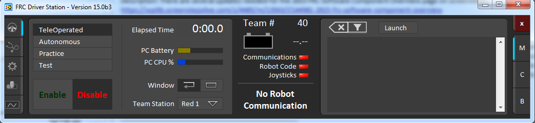
This is the only software allowed to be used for the purpose of controlling the state of the robot during competition. This software sends data to your robot from a variety of input devices. It also contains a number of tools used to help troubleshoot robot issues. More information about the FRC Driver Station Powered by NI LabVIEW can be found here.
Dashboard Options
LabVIEW Dashboard (Windows Only)
The LabVIEW Dashboard is automatically launched by the FRC Driver Station by default. The purpose of the Dashboard is to provide feedback about the operation of the robot using tabbed display with a variety of built in features. More information about the FRC Default Dashboard software can be found here.
SmartDashboard

SmartDashboard allows you to view your robot data by automatically creating customizable indicators specifically for each piece of data sent from your robot. Additional documentation on SmartDashboard can be found here.
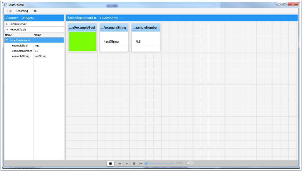
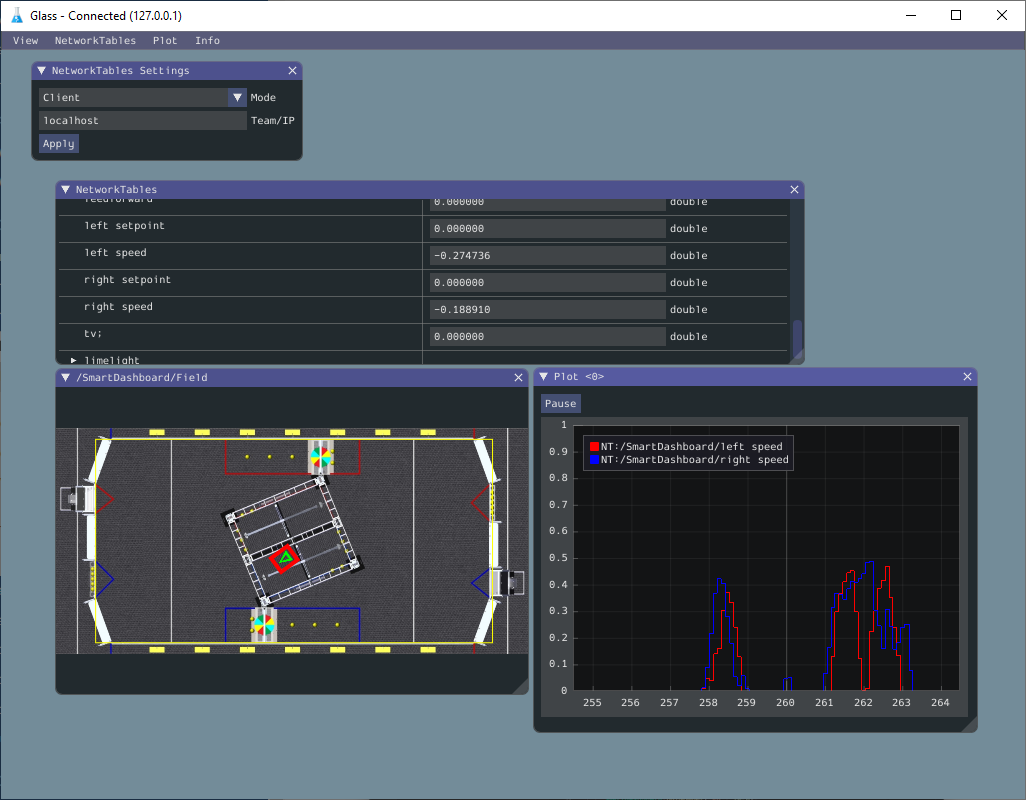
LiveWindow
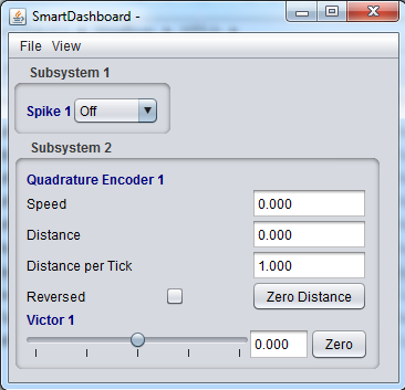
LiveWindow is a feature of SmartDashboard and Shuffleboard, designed for use with the Test Mode of the Driver Station. LiveWindow allows the user to see feedback from sensors on the robot and control actuators independent of the written user code. More information about LiveWindow can be found here.
FRC roboRIO Imaging Tool (Windows Only)
This tool is used to format and setup a roboRIO for use in FRC. Installation instructions can be found here. Additional instructions on imaging your roboRIO using this tool can be found here.
FRC Radio Configuration Utility (Windows Only)
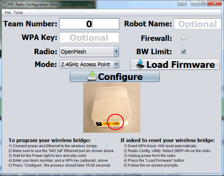
The FRC Radio Configuration Utility is a tool used to configure the standard radio for practice use at home. This tool sets the appropriate network settings to mimic the experience of the FRC playing field. The FRC Radio Configuration Utility is installed by a standalone installer that can be found here.
FRC Driver Station Log Viewer (Windows Only)
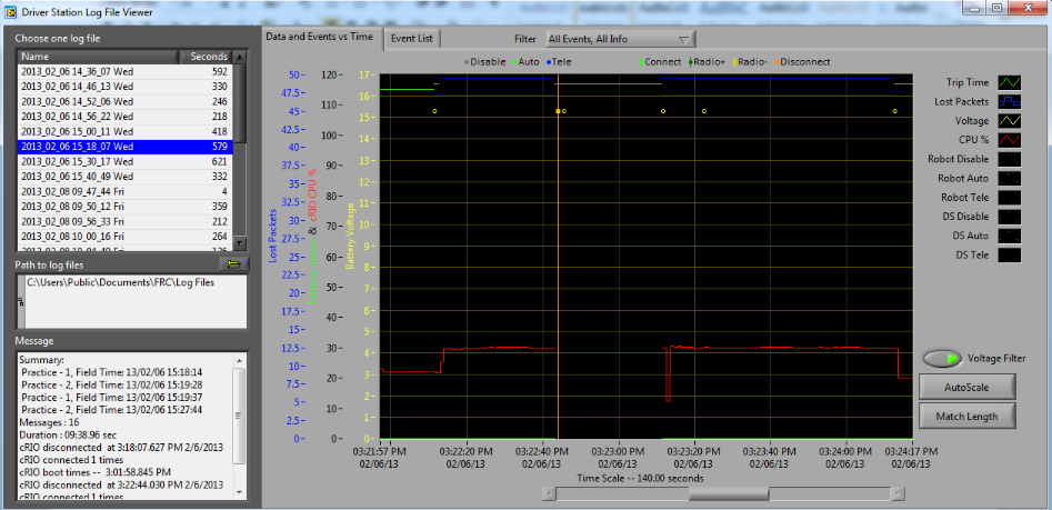
The FRC Driver Station Log Viewer is used to view logs created by the FRC Driver Station. These logs contain a variety of information important for understanding what happened during a practice session or FRC match. More information about the FRC Driver Station Log Viewer and understanding the logs can be found here
RobotBuilder
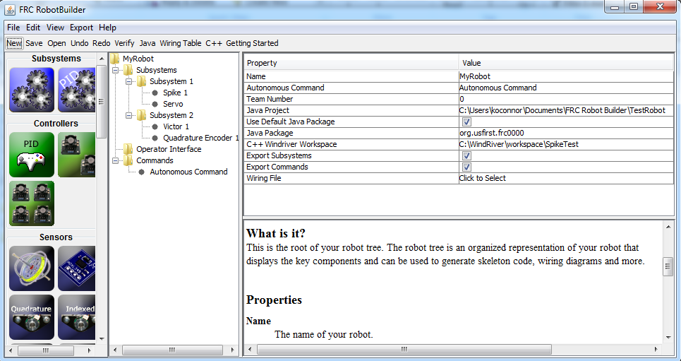
RobotBuilder is a tool designed to aid in setup and structuring of a Command Based robot project for C++ or Java. RobotBuilder allows you to enter in the various components of your robot subsystems and operator interface and define what your commands are in a graphical tree structure. RobotBuilder will then generate structural template code to get you started. More information about RobotBuilder can be found here. More information about the Command Based programming architecture can be found here.
Robot Simulation
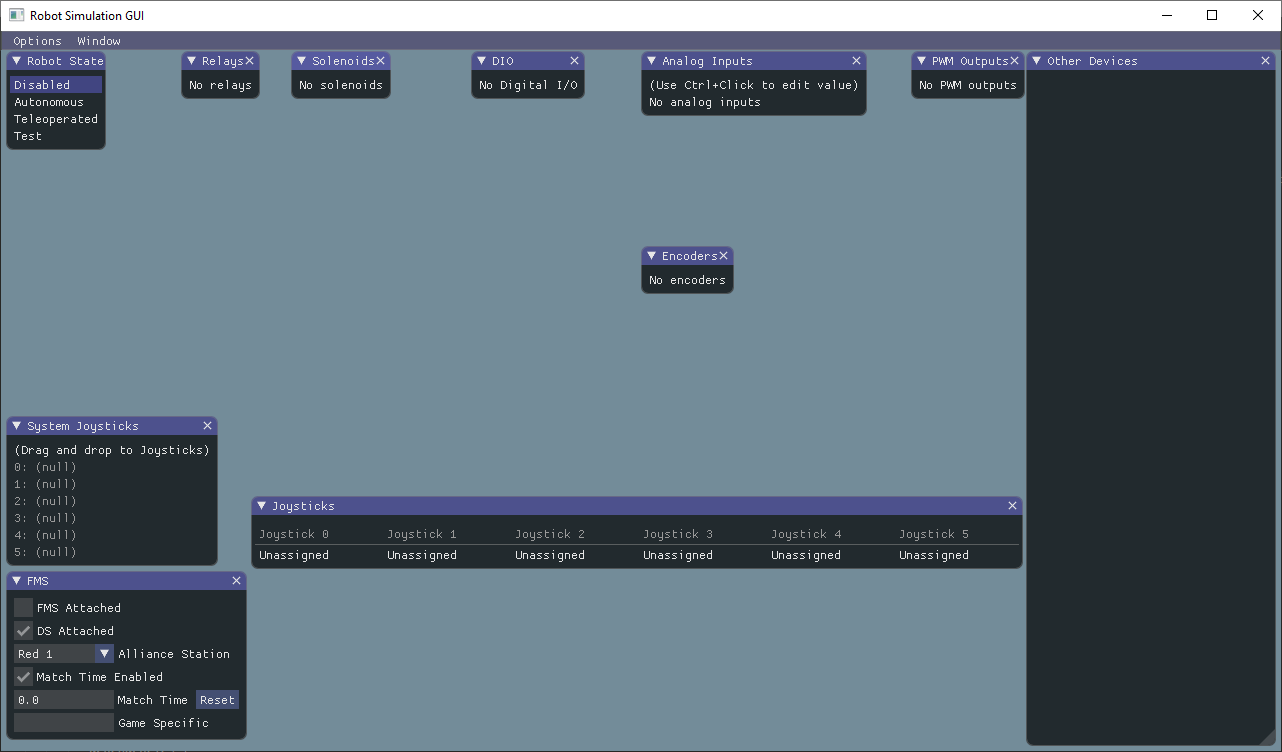
Robot Simulation offers a way for Java and C++ teams to verify their actual robot code is working in a simulated environment. This simulation can be launched directly from VS Code and includes a 2D field that users can visualize their robot’s movement on. For more information see the Robot Simulation section.
FRC LabVIEW Robot Simulator (Windows Only)
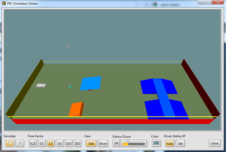
The FRC Robot Simulator is a component of the LabVIEW programming environment that allows you to operate a predefined robot in a simulated environment to test code and/or Driver Station functions. Information on using the FRC Robot Simulator can be found here or by opening the Robot Simulation Readme.html file in the LabVIEW Project Explorer.
PathWeaver
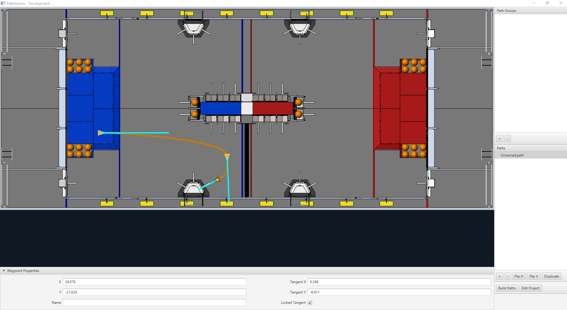
PathWeaver allows teams to quickly generate and configure paths for advanced autonomous routines. These paths have smooth curves allowing the team to quickly navigate thir robot between points on the field. For more information see the PathWeaver section.
Robot Characterization
This tool helps teams automatically calculate constants that can be used to describe the physical properties of your robot for use in features like robot simulation, trajectory following, and PID control. For more information see the Robot Characterization section.
OutlineViewer
OutlineViewer is a utility used to view, modify and add to all of the contents of the NetworkTables for debugging purposes. LabVIEW teams can use the Variables tab of the LabVIEW Dashboard to accomplish this functionality. For more information see the Outline Viewer section.
Setup Axis Camera (Windows Only)
The Setup Axis Camera utility is a LabVIEW program used to configure an Axis 206, M1011 or M1013 camera for use on the robot. The Setup Axis Camera tool is installed as part of the FRC Game Tools.
What is WPILib?
The WPI Robotics Library (WPILib) is the standard software library provided for teams to write code for their FRC® robots. A software library is a collection of code that can be imported into and used by other software. WPILib contains a set of useful classes and subroutines for interfacing with various parts of the FRC control system (such as sensors, motor controllers, and the driver station), as well as an assortment of other utility functions.
Supported languages
There are two versions of WPILib, one for each of the two officially-supported text-based languages: WPILibJ for java, and WPILibC for C++. A considerable effort is made to maintain feature-parity between these two languages - library features are not added unless they can be reasonably supported for both Java and C++, and when possible the class and method names are kept identical or highly-similar. While unofficial community-built support is available for some other languages, notably python, this documentation will only cover Java and C++. Java and C++ were chosen for the officially-supported languages due to their appropriate level-of-abstraction and ubiquity in both industry and high-school computer science classes.
In general, C++ offers better high-end performance, at the cost of increased user effort (memory must be handled manually, and the C++ compiler does not do much to ensure user code will not crash at runtime). Java offers lesser performance, but much greater convenience. New/inexperienced users are strongly encouraged to use Java.
Source code and documentation
WPILib is an open-source library - the entirety of its source code is available online on the WPILib GitHub Page:
The Java and C++ source code can be found in the WPILibJ and WPILibC source directories:
While users are strongly encouraged to read the source code to resolve detailed questions about library functionality, more-concise documentation can be found on the official documentation pages for WPILibJ and WPILibC:
2022 Overview
Known Issues
This article details known issues (and workarounds) for FRC® Control System Software.
Open Issues
Onboard I2C Causing System Lockups
Issue: Use of the onboard I2C port, in any language, can result in system lockups. The frequency of these lockups appears to be dependent on the specific hardware (i.e. different roboRIOs will behave differently) as well as how the bus is being used.
Workaround: The only surefire mitigation is to use the MXP I2C port instead. Acessing the device less frequently and/or using a different roboRIO may significantly reduce the likelihood/frequency of lockups, it will be up to each team to assess their tolerance of the risk of lockup. This lockup can not be definitively identified on the field and a field fault will not be called for a match where this behavior is believed to occur. This lockup is a CPU/kernel hang, the roboRIO will completely stop responding and will not be accessible via the DS, webpage or SSH. If you can access your roboRIO via any of these methods, you are experiencing a different issue.
Analog Devices Gyros don’t work properly
Issue: Due to an issue with the “autoSPI” feature in the roboRIO image 2022_v3.0, Analog Devices gyros do not work properly.
Workaround: There is no known workaround. An updated image will be released when the issue has been resolved.
Game Tools Autorun graphics say 2020
Issue: If you launch the Game Tools installer by using the Autorun file, the menu item correctly says 2022, but the graphic says 2020.
Workaround: This can be safely ignored, if the menu item says 2022, you are installing the correct software.
Updating Properties on roboRIO 2.0 may be slow or hang
Issue: Updating the properties on a roboRIO 2.0 without reformatting using the Imaging Tool (such as setting the team number) may be slow or hang.
Workaround: After a few minutes of the tool waiting the roboRIO should be able to be rebooted and the new properties should be set.
Invalid build due to missing GradleRIO
Issue: Rarely, a user’s Gradle cache will get broken and they will get shown errors similar to the following:
Could not apply requested plugin [id: ‘edu.wpi.first.GradleRIO’, version: ‘2020.3.2’] as it does not provide a plugin with id ‘edu.wpi.first.GradleRIO’
Workaround:
Delete your Gradle cache located under ~$USER_HOME/.gradle. Windows machines may need to enable the ability to view hidden files. This issue has only shown up on Windows so far. Please report this issue if you get it on an alternative OS.
Unable to Build Robot Projects outside of VS Code on M1-based macOS
Issue: Error when building a robot project in non-WPILib installations.
Could not determine the dependencies of task ':extractReleaseNative'.
> Could not resolve all files for configuration ':nativeRelease'.
  > Failed to transform hal-cpp-2022.1.1-rc-1-osxx86.zip (edu.wpi.first.hal:hal-cpp:2022.1.1-rc-1) to match attributes {artifactType=gr-directory, org.gradle.status=release}.
...
Workaround: M1-based macOS is not supported. The above error will show up when using an ARM-based JDK. User must use a x64-compatible JDK 11 or preferably use the WPILib installer.
Chinese characters in Driver Station Log
Issue: Rarely, the driver station log will show Chinese characters instead of the English text. This appears to only happen when Windows is set to a language other then English.
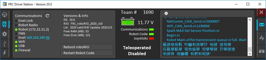
Workaround: There are two known workarounds:
Copy and paste the Chinese characters into notepad, and the English text will be shown.
Temporarily change the Windows language to English.
C++ Intellisense - Files Open on Launch Don’t Work Properly
Issue: In C++, files open when VS Code launches will have issues with Intellisense showing suggestions from all options from a compilation unit and not just the appropriate ones or not finding header files. This is a bug in VS Code.
Workaround:
Close all files in VS Code, but leave VS Code open
Delete c_cpp_properties.json file in the .vscode folder, if it exists
Run the “Refresh C++ Intellisense” command in vscode.
In the bottom right you should see something that looks like a platform (linuxathena or windowsx86-64 etc). If it’s not linuxathena click it and set it to linuxathena (release)
Wait ~1 min
Open the main cpp file (not a header file). Intellisense should now be working
Issues with WPILib Dashboards and Simulation on Windows N Editions
Issue: WPILib code using CSCore (dashboards and simulated robot code) will have issues on Education N editions of Windows.
Shuffleboard will run, but not load cameras
Smartdashbard will crash on start-up
Robot Simulation will crash on start-up
Solution: Install the Media Feature Pack
NetworkTables Interoperability
There is currently an issue with inter-operating C++/Java NetworkTables clients (dashboards or co-processors) with LabVIEW servers (LV robot code). In some scenarios users will see updates from one client fail to be replicated across to other clients (e.g. data from a co-processor will not be properly replicated out to a dashboard). Data still continues to return correctly when accessed by code on the server.
Workaround: Write code on the server to mirror any keys you wish to see on other clients (e.g. dashboards) to a separate key. For example, if you have a key named targetX being published by a co-processor that you want to show up on a dashboard, you could write code on the robot to read the key and re-write it to a key like targetXDash.
Fixed in WPILib 2022.2.1
Joysticks may stop updating in Java
Issue: A deadlock in the Java WPILib DriverStation thread may occur. This is primarily noticeable by Joystick values “freezing” and not updating. Disable and E-Stop are not affected by this issue.
Recommendations: Ensure that anyone operating a robot is prepared to disable or E-Stop if this issue occurs. Limit calls to the following DriverStation methods: isEnabled, isEStopped, isAutonomous, isDisabled, isAutonomousEnabled, isTeleopEnabled, isTest, isDSAttached, isFMSAttached, and updateControlWord, especially from multiple threads, to limit the chance of the deadlock occurring. Follow this WPILib issue for more updates and possible workarounds.
VS Code Vendor Check for Updates Broken
Issue: Checking for vendor library updates online results in the following error message: Command ‘WPILib: Manage Vendor Libraries’ resulted in an error (Only absolute URLs are supported). This is caused by a bug in the VS Code extension related to the way the WPILib Command library vendordeps were created. This issue will be fixed in the next WPILib release.
Workaround: If you aren’t using either the new or old Command vendordep, remove them from your project. Alternately, the new or old Command vendordep can be temporarily removed before checking for updates, and then re-added.
Shuffleboard aborts while launching
Issue: Shuffleboard may start to open, and then abort. This is caused by issues with the scripts for launching the WPILib tools.
Workaround: Manually launch Shuffleboard from the commandline without using the shortcut or script. On Windows run c:\Users\Public\wpilib\2022\jdk\bin\java -jar c:\Users\Public\wpilib\2022\tools\shuffleboard.jar. On Linux or macOS, run ~/wpilib/2022/jdk/bin/java -jar ~/wpilib/2022/tools/shuffleboard.jar
Note
This issue may affect any WPILib java tool, as they use the same scripts to open. If you have issues with PathWeaver, RobotBuilder, or SmartDashboard replace shuffleboard.jar above with PathWeaver.jar, RobotBuilder.jar or SmartDashboard.jar
New for 2022
Important
Due to the large number of breaking and substantial changes between 2021 and 2022, it is advised that existing teams thoroughly read this document!
A number of improvements have been made to FRC® Control System software for 2022. This article will describe and provide a brief overview of the new changes and features as well as a more complete changelog for Java/C++ WPILib changes. This document only includes the most relevant changes for end users, the full list of changes can be viewed on the various WPILib GitHub repositories. WPILib recognizes that some of these changes may cause teams issues in the short term upgrading. We expect it to pay off over the long term as we better improve the internals of WPILib.
Due to internal GradleRIO changes, it is necessary to update previous years projects. After Installing WPILib for 2022, any 2020 or 2021 projects must be imported to be compatible.
It’s recommended to also review the list of known issues.
Major Changes (Java/C++)
These changes contain some of the major changes to the library that it’s important for the user to recognize. This does not include all of the breaking changes, see the other sections of this document for more changes.
Drive class functions such as
DifferentialDriveandMecanumDriveno longer invert the right side by default. Please usesetInvertedon your motor controllers to invert the right side to maintain the same behaviorOld Command-Based has been removed from the list of new templates in VS Code. Please migrate to the new Command-Based library. The Old Command Based remains available to support existing code.
IterativeRobot has been removed. Please use the TimedRobot template instead
WPILib
General Library
Rewrite Mechanism2d to utilize NetworkTables
Improved the error message when a program crashes
Added support for DMA to Java
Added
TimesliceRobotproject template. This allows users to timeslice schedule periodic functionsAdded C++ TankDrive example
Added
PS4Controllercontroller classAdded better message for when an I2C port is out of range
Added
Debouncer(Java, C++) class. This helps with filtering rising and falling edges when dealing with boolean valuesAdded
PneumaticHubclass for use with the REV Pneumatic HubGenericHID has been updated to static functions to use for non-defined controller types.
XboxControllerhas migrated away from taking arguments in functions and instead has functions with no arguments. An example conversion is below:controller.getTriggerAxis(GenericHID.Hand.kLeft)->controller.getLeftTriggerAxis()controller.getX(GenericHID.Hand.kLeft)->controller.getLeftX()
getInstance()functions inCameraServer,DriverStation,LiveWindow,Preferences,SendableRegistry, have been deprecated and replaced with static functionsTimer::HasPeriodPassed()andTimer.hasPeriodPassed()have been deprecated. UseAdvanceIfElapsed()insteadSeveral new classes have been added to enable simpler access to
Counter:ExternalDirectionCounter(Java/ C++),Tachometer(Java/ C++), andUpDownCounter(Java/ C++)DutyCycleEncoder: add support for setting duty cycle rangeAdded
ADIS16448_IMUandADIS16470_IMUclasses.Added
BangBangControllerclass (Java, C++) for maximally-aggressive velocity control of high-inertia mechanisms, which is useful for flywheel shooters.
Breaking Changes
PDPis nowPowerDistributionVarious
PCMrelated classes (Solenoid, Compressor) now require aPneumaticsModuleTypeto support either the CTRE Pneumatics Control Module or REV Pneumatic Hub. Vendor specific methods have been moved to thePneumaticsControlModuleorPneumaticHubclassesSendable has been broken up into NetworkTables components (called NTSendable*,
ntnamespace) and non-NetworkTables components (moved to wpiutil,wpinamespace). This will make it easier for vendors and external libraries to integrate SendableInterruptableSendableBasehas been broken up intoAsynchronousInterrupt&SynchronousInterrupt. Rather then a class, likeDigitalInputextendingInterruptableSendableBaseand all interrupt methods being accessed through theDigitalInput, teams should instead constructAsynchronousInterruptorSynchronousInterrupt, and pass it theDigitalSource(e.g.DigitalInput).C++:
DriverStation.ReportWarningandDriverStation.ReportErrorhave been removed. UseFRC_ReportErrorinfrc\Errors.hheader. Status offrc::err::Errorcan be used for Errors andfrc::warn::Warningcan be used for warnings.SpeedControllerhas been renamed toMotorControllerVarious portions of the API still refers to
SpeedControllerfor backwards compatibility. Users should passMotorControllerinstead
Several duplicate
SpeedControllermethods have been removed. Usesetinstead ofsetSpeed. Usedisableinstead ofsetDisable. Several low level methods have been removed: position, bounds, periodMultiplier, zeroLatch, and raw methods. Use thePWMclass directly if this level of control is needed.Various DriverStation In[Mode] functions has been renamed (IE:
InDisabled->inDisabled)Deprecated
wpilibj.cameraserverhas been removed. UsecameraserverinsteadDeprecated
RobotDrivehas been removed. UseDifferentialDriveinsteadDeprecated
GearToothhas been removed. Use theCounterclass insteadC++: Deprecated
WPILib.hhas been removed. Please only include what you needC++:
wpi::StringRefis replaced withstd::string_view. This is a drop in replacement in most casesC++:
wpi::ArrayRefis replaced withwpi::span. This is a modified backport of the C++20std::spanC++:
wpi::Twineis replaced with fmtlib. It has more features and is standard in C++20C++:
wpi::sys::pathis replaced withfs::pathfrom#include <wpi/fs.h>which is based onstd::filesystemC++:
frc::filesystemmethods have been simplified to returnstd::string, rather then using a pointer parameterC++:
wpi::mathis replaced withwpi::numberswhich is based on C++20std::numbers.C++: Support for
std::coutwas removed from units because<iostream>has significant compile-time overhead. Use fmtlib instead, an analog for C++20’sstd::format()(e.g.,fmt::print("{}", 2_m)). The units headers automatically include fmtlib. If you still want to usestd::cout, callvalue()on the variable being printed (e.g.,std::cout << velocity.value()).C++: Various classes have migrated to use units:
Ultrasonic,CommandScheduler,CommandState,WaitUntilCommand,MecanumControllerCommand,RamseteCommand,SwerveControllerCommand,TrapezoidProfileCommand,WaitCommand,Counter,CounterBase,DriverStation,Encoder,InterruptableSensorBase,MotorSafety,Notifier,SPI,SerialPort,SlewRateLimiter,Solenoid,Timer,Watchdog, and Old Commands:Command,CommandGroup,CommandGroupEntry,TimedCommand,WaitCommand,WaitForChildren,WaitUntilCommandThe old
PIDController,PIDSourceandPIDOutputclasses have been moved from the main library to the Old Commands Vendordep. Wrapper classes in the pidwrappers package have been added for PIDSource and PIDoutput support for WPILib classes, also in the Old Commands Vendordep. These classes have been deprecated since 2020. The new PID Controller inedu.wpi.first.math.controllerfor Java andfrc2for C++ is the recommended replacement.PreferencesputX methods (e.g. putDouble) have been deprecated and replaced with setX methods for consistency with the rest of WPILib API.
Package Renames
We have committed to several organizational renames that will allow us greater flexible with new classes in the future. The VS Code project importer will update existing projects to use the new packages/headers.
Several packages moved from
wpilibjtomath:controller,estimator,geometry,kinematics,math,spline,system,trajectorywpiutil.mathwas moved tomathwpiutilis nowutilSlewRateLimiter,LinearFilter, andMedianFilternow live inmath.filters, along with the newly-addedDebouncer.Timerhas moved fromfrc2tofrcMotor controllers (
VictorSPX,PWMSparkMax, etc) have been moved to amotorcontrolpackage.edu.wpi.cscorehas moved toedu.wpi.first.cscore
Simulation
Uses multi-file
jsonsave formats instead ofiniand supports loading/saving the workspace; when started from the VS Code tool menu, these default to using the project directory for saving rather than the system-global location
Shuffleboard
Add widget for
Field2dAdd icons to widget layouts
Add titles for widgets
Show exit save prompt only if not saved
Use system menubar
Add tab clear confirmation
Save widget titles display mode preference
Fix: CameraServer streams
Fix: Shuffleboard not starting on Windows N. Media Feature Pack is still needed for camera support.
SmartDashboard
No new changes
Glass
Uses multi-file
jsonsave formats instead ofiniand supports loading/saving the workspace; when started from the VS Code tool menu, these default to using the project directory for saving rather than the system-global location
Axon
We have made a new tool for machine learning in the FIRST Robotics Competition. Axon allows users to view and create datasets, train machine learning models, test your models within the browser-based GUI, and export them for use on a Raspberry Pi. Detecting complex objects (such as hatch panels and other robots) has never been easier and an end-to-end user guide is available in the WPILib docs. Axon provides the functionality to train machine learning models to recognize any object you want (defined in a homemade dataset), or generic objects such as cats, airplanes, and hot dogs.
Axon is a replacement for the previous AWS-based Jupyter Notebook solution released in the 2019 season. Axon has a smooth installation and user experience overall, and a much more friendly GUI for beginners and experts alike.
Running machine learning models on the WPILib Raspberry Pi image has never been easier either; the new Python script for the Pi features time-synchronous NetworkTables data streaming, as well as a better quality live inference MJPEG stream.
PathWeaver
No new changes
GradleRIO
Gradle has been updated to version 7.3.2
Internals of GradleRIO have been updated to be easier to read, more maintainable and easier for advanced teams to modify.
Deployment is more customizable
cscore
The supported OpenCV version has been bumped to OpenCV4
OutlineViewer
OutlineViewer has been updated to be C++ based using the ImGui library. This makes OutlineViewer more maintainable and performant.
Important
The Java version of OutlineViewer is discontinued and is no longer supported!
WPILib All in One Installer
Simplified installation choices
Visual Studio Code has been updated to 1.63.2
Updated Java and C++ language extensions
Fix Linux desktop icon permissions
Add year to tools shortcuts name
Handle issues with JDK running and UAC canceled
Visual Studio Code Extension
Important
The project importer will only import 2020/2021 projects!
Project Importer has been updated for the 2022 season. The project importer will attempt update the imported code, but manual changes may still be necessary due to the complexity of the breaking changes this year.
Remove Eclipse Project Importer
Fix chcp not found warning during simulation on Windows
Add additional information to the project information command display
RobotBuilder
Important
Due to project file changes, Robotbuilder will not import yaml save files from 2021 or earlier.
Update to compile with WPILib 2022 (remove RobotDrive and GearTooth), update PID Controllers, and pneumatics
Improve type detection to detect changes in certain C++ types that were not previously detected as changes
Add project setting to enable or disable desktop support
Fix Java export of DoubleSolenoid, RobotDrive4, MecanumDrive, and Killough drive to avoid extra local copy
Fix C++ export of ConditionalCommand
Don’t validate timeout parameters that are less than 0
SysID
SysId is a fully featured system characterization utility that supersedes frc-characterization. It features an easy-to-use interface, advanced graphing analytics, Romi integration and other cool features!.
Important
frc-characterization is discontinued and is no longer supported!
Romi
A Romi Library has been created to contain several helper classes that are a part of the
RomiReferenceexample. Romi Vendordep.
VS Code Overview
Visual Studio Code Basics and the WPILib Extension
Microsoft’s Visual Studio Code is the supported IDE for C++ and Java development in FRC. This article introduces some of the basics of using Visual Studio Code and the WPILib extension.
Welcome Page
When Visual Studio Code first opens, you are presented with a Welcome page. On this page you will find some quick links that allow you to customize Visual Studio Code as well as a number of links to help documents and videos that may help you learn about the basics of the IDE as well as some tips and tricks.
You may also notice a small WPILib logo way up in the top right corner. This is one way to access the features provided by the WPILib extension (discussed further below).
User Interface
The most important link to take a look at is probably the basic User Interface document. This document describes a lot of the basics of using the UI and provides the majority of the information you should need to get started using Visual Studio Code for FRC.
Command Palette
The Command Palette can be used to access or run almost any function or feature in Visual Studio Code (including those from the WPILib extension). The Command Palette can be accessed from the View menu or by pressing Ctrl+Shift+P (Cmd+Shift+P on macOS). Typing text into the window will dynamically narrow the search to relevant commands and show them in the dropdown.
In the following example “wpilib” is typed into the search box after activating the Command Palette, and it narrows the list to functions containing WPILib.
WPILib Extension
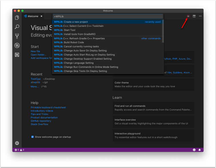
The WPILib extension provides the FRC® specific functionality related to creating projects and project components, building and downloading code to the roboRIO and more. You can access the WPILib commands one of two ways:
By typing “WPILib” into the Command Palette
By clicking on the WPILib icon in the top right of most windows. This will open the Command Palette with “WPILib” pre-entered
Note
It is not recommended to install the Visual Studio IntelliCode plugin with the FRC installation of VS Code as it is known to break IntelliSense in odd ways.
For more information about specific WPILib extension commands, see the other articles in this chapter.
WPILib Commands in Visual Studio Code
This document contains a complete list of the commands provided by the WPILib VS Code Extension and what they do.
To access these commands, press Ctrl+Shift+P to open the Command Palette, then begin typing the command name as shown here to filter the list of commands. Click on the command name to execute it.
WPILib: Build Robot Code - Builds open project using GradleRIO
WPILib: Create a new project - Create a new robot project
WPILib C++: Refresh C++ Intellisense - Force an update to the C++ Intellisense configuration.
WPILib C++: Select current C++ toolchain - Select the toolchain to use for Intellisense (i.e. desktop vs. roboRIO vs…). This is the same as clicking the current mode in the bottom right status bar.
WPILib C++ Select Enabled C++ Intellisense Binary Types - Switch Intellisense between static, shared, and executable
WPILib: Cancel currently running tasks - Cancel any tasks the WPILib extension is currently running
WPILib: Change Auto Save On Deploy Setting - Change whether files are saved automatically when doing a Deploy. This defaults to Enabled.
WPILib: Change Auto Start RioLog on Deploy Setting - Change whether RioLog starts automatically on deploy. This defaults to Enabled.
WPILib: Change Desktop Support Enabled Setting - Change whether building robot code on Desktop is enabled. Enable this for test and simulation purposes. This defaults to Desktop Support off.
WPILib: Change Language Setting - Change whether the currently open project is C++ or Java.
WPILib: Change Run Commands Except Deploy/Debug in Offline Mode Setting - Change whether GradleRIO is running in Online Mode for commands other then deploy/debug (will attempt to automatically pull dependencies from online). Defaults to enabled (online mode).
WPILib: Change Run Deploy/Debug Command in Offline Mode Setting - Change whether GradleRIO is running in Online Mode for deploy/debug (will attempt to automatically pull dependencies from online). Defaults to disabled (offline mode).
WPILib: Change Select Default Simulate Extension Setting - Change whether simulation extensions are enabled by default (all simulation extensions defined in
build.gradlewill be enabled)WPILib: Change Skip Tests On Deploy Setting - Change whether to skip tests on deploy. Defaults to disabled (tests are run on deploy)
WPILib: Change Stop Simulation on Entry Setting - Change whether to stop robot code on entry when running simulation. Defaults to disabled (don’t stop on entry).
WPILib: Check for WPILib Updates - Check for an update to the WPILib extensions
WPILib: Debug Robot Code - Build and deploy robot code to roboRIO in debug mode and start debugging
WPILib: Deploy Robot Code - Build and deploy robot code to roboRIO
WPILib: Import a WPILib 2020/2021 Gradle Project - Open a wizard to help you create a new project from a existing VS Code Gradle project from 2020 or 2021. Further documentation is at importing gradle project
WPILib: Install tools from GradleRIO - Install the WPILib Java tools (e.g. SmartDashboard, Shuffleboard, etc.). Note that this is done by default by the offline installer
WPILib: Manage Vendor Libraries - Install/update 3rd party libraries
WPILib: Open API Documentation - Opens either the WPILib Javadocs or C++ Doxygen documentation
WPILib: Open Project Information - Opens a widget with project information (Project version, extension version, etc.)
WPILib: Open WPILib Command Palette - This command is used to open a WPILib Command Palette (equivalent of hitting Ctrl+Shift+P and typing
WPILib)WPILib: Open WPILib Help - This opens a simple page which links to the WPILib documentation (this site)
WPILib: Reset Ask for WPILib Updates Flag - This will clear the flag on the current project, allowing you to re-prompt to update a project to the latest WPILib version if you previously chose to not update.
WPILib: Run a command in Gradle - This lets you run an arbitrary command in the GradleRIO command environment
WPILib: Set Team Number - Used to modify the team number associated with a project. This is only needed if you need to change the team number from the one initially specified when creating the project.
WPILib: Set VS Code Java Home to FRC Home - Set the VS Code Java Home variable to point to the Java Home discovered by the FRC extension. This is needed if not using the offline installer to make sure the intellisense settings are in sync with the WPILib build settings.
WPILib: Show Log Folder - Shows the folder where the WPILib extension stores internal logs. This may be useful when debugging/reporting an extension issue to the WPILib developers
WPILib: Simulate Robot Code on Desktop - This builds the current robot code project on your PC and starts it running in simulation. This requires Desktop Support to be set to Enabled.
WPILib: Start RioLog - This starts the RioLog display used to view console output from a robot program
WPILib: Start Tool - This allows you to launch WPILib tools (e.g. SmartDashboard, Shuffleboard, etc.) from inside VS Code
WPILib: Test Robot Code - This builds the current robot code project and runs any created tests. This requires Desktop Support to be set to Enabled.
Creating a Robot Program
Once everything is installed, we’re ready to create a robot program. WPILib comes with several templates for robot programs. Use of these templates is highly recommended for new users; however, advanced users are free to write their own robot code from scratch.
Choosing a Base Class
To start a project using one of the WPILib robot program templates, users must first choose a base class for their robot. Users subclass these base classes to create their primary Robot class, which controls the main flow of the robot program. There are three choices available for the base class:
TimedRobot
The TimedRobot class is the the base class recommended for most users. It provides control of the robot program through a collection of init(), periodic(), and exit() methods, which are called by WPILib during specific robot states (e.g. autonomous or teleoperated). The TimedRobot class also provides an example of retrieving autonomous routines through SendableChooser (Java/ C++
Note
A TimedRobot Skeleton template is available that removes some informative comments and the autonomous example. You can use this if you’re already familiar with TimedRobot. The example shown below is of TimedRobot Skeleton.
import edu.wpi.first.wpilibj.TimedRobot;

public class Robot extends TimedRobot {

    @Override
    public void robotInit() {
        // This is called once when the robot code initializes
    }

    @Override
    public void robotPeriodic() {
        // This is called every period regardless of mode
    }

    @Override
    public void autonomousInit() {
        // This is called once when the robot first enters autonomous mode
    }

    @Override
    public void autonomousPeriodic() {
        // This is called periodically while the robot is in autonomous mode
    }

    @Override
    public void teleopInit() {
        // This is called once when the robot first enters teleoperated mode
    }

    @Override
    public void teleopPeriodic() {
        // This is called periodically while the robot is in teleoperated mode
    }

    @Override
    public void testInit() {
        // This is called once when the robot enters test mode
    }

    @Override
    public void testPeriodic() {
        // This is called periodically while the robot is in test mode
    }

}
#include <frc/TimedRobot.h>

class Robot : public frc::TimedRobot {
    public:
        void RobotInit() override; // This is called once when the robot code initializes
        void RobotPeriodic() override; // This is called every period regardless of mode
        void AutonomousInit() override; // This is called once when the robot first enters autonomous mode
        void AutonomousPeriodic() override; // This is called periodically while the robot is in autonomous mode
        void TeleopInit() override; // This is called once when the robot first enters teleoperated mode
        void TeleopPeriodic() override; // This is called periodically while the robot is in teleoperated mode
        void TestInit() override; // This is called once when the robot enters test mode
        void TestPeriodic() override; // This is called periodically while the robot is in test mode
};
Periodic methods are called every 20 ms by default. This can be changed by calling the superclass constructor with the new desired update rate.
Danger
Changing your robot rate can cause some unintended behavior (loop overruns). Teams can also use Notifiers to schedule methods at a custom rate.
public Robot() {
  super(0.03); // Periodic methods will now be called every 30 ms.
}
Robot() : frc::TimedRobot(30_ms) {}
RobotBase
The RobotBase class is the most minimal base-class offered, and is generally not recommended for direct use. No robot control flow is handled for the user; everything must be written from scratch inside the startCompetition() method. The template by default showcases how to process the different operation modes (teleop, auto, etc).
Note
A RobotBase Skeleton template is available that offers a blank startCompetition() method.
Command Robot
Teams using Command Robot should see the Command-Based Programming Tutorial.
Romi
Teams using a Romi should use the Romi - Timed or Romi - Command Bot template.
Romi - Timed
The Romi - Timed template provides a RomiDrivetrain class that exposes an arcadeDrive(double xaxisSpeed, double zaxisRotate) method. It’s up to the user to feed this arcadeDrive function.
This class also provides functions for retrieving and resetting the Romi’s onboard encoders.
Romi - Command Bot
The Romi - Command Bot template provides a RomiDrivetrain subsystem that exposes an arcadeDrive(double xaxisSpeed, double zaxisRotate) method. It’s up to the user to feed this arcadeDrive function.
This subsystem also provides functions for retrieving and resetting the Romi’s onboard encoders.
Not Using a Base Class
If desired, users can omit a base class entirely and simply write their program in a main() method, as they would for any other program. This is highly discouraged - users should not “reinvent the wheel” when writing their robot code - but it is supported for those who wish to have absolute control over their program flow.
Warning
Users should not modify the main() method of a robot program unless they are absolutely sure of what they are doing.
Creating a New WPILib Project
Once we’ve decided on a base class, we can create our new robot project. Bring up the Visual Studio Code command palette with Ctrl+Shift+P:
Then, type “WPILib” into the prompt. Since all WPILib commands start with “WPILib,” this will bring up the list of WPILib-specific VS Code commands:
Now, select the Create a new project command:
This will bring up the “New Project Creator Window:”
The elements of the New Project Creator Window are explained below:
Project Type: The kind of project we wish to create. This can be an example project, or one of the project templates provided by WPILib. Templates exist for each of the robot base classes. Additionally, a template exists for Command-based projects, which are built on the
TimedRobotbase class but include a number of additional features - this type of robot program is highly recommended for new teams.Language: This is the language (C++ or Java) that will be used for this project.
Base Folder: If this is a template project, this specifies the type of template that will be used.
Project Location: This determines the folder in which the robot project will be located.
Project Name: The name of the robot project. This also specifies the name that the project folder will be given if the Create New Folder box is checked.
Create a New Folder: If this is checked, a new folder will be created to hold the project within the previously-specified folder. If it is not checked, the project will be located directly in the previously-specified folder. An error will be thrown if the folder is not empty and this is not checked.
Team Number: The team number for the project, which will be used for package names within the project and to locate the robot when deploying code.
Enable Desktop Support: Enables unit test and simulation. While WPILib supports this, third party software libraries may not. If libraries do not support desktop, then your code may not compile or may crash. It should be left unchecked unless unit testing or simulation is needed and all libraries support it.
Once all the above have been configured, click “Generate Project” and the robot project will be created.
Note
Any errors in project generation will appear in the bottom right-hand corner of the screen.
An example after all options are selected is shown below.
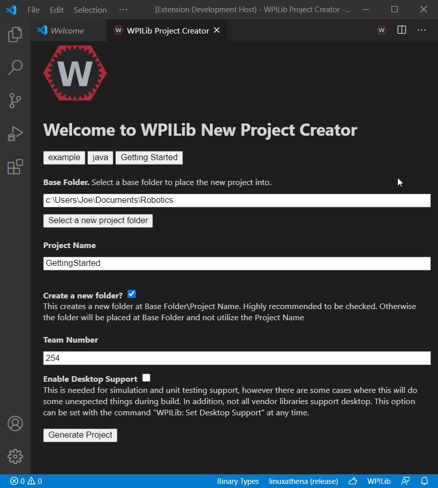
Opening The New Project
After successfully creating your project, VS Code will give the option of opening the project as shown below. We can choose to do that now or later by typing Ctrl+K then Ctrl+O (or just Command+O on macOS) and select the folder where we saved our project.
Once opened we will see the project hierarchy on the left. Double clicking on the file will open that file in the editor.
C++ Configurations (C++ Only)
For C++ projects, there is one more step to set up IntelliSense. Whenever we open a project, we should get a pop-up in the bottom right corner asking to refresh C++ configurations. Click “Yes” to set up IntelliSense.
3rd Party Libraries
Teams that are not using parts provided in the KoP will likely need to install external dependencies. Please view the below section to see information on adding an external library.
The Mechanism
In support of this effort NI (for LabVIEW) and FIRST/WPI (for Java/C++) have developed mechanisms that should make it easy for vendors to plug their code into the WPILib software and for teams to use that code once it has been installed. A brief description of how the system works for each language can be found below.
The Mechanism - Java/C++
For Java and C++ a JSON file describing the vendor library is installed on your system to ~/wpilib/YYYY/vendordeps (where YYYY is the year and ~ is C:\Users\Public on Windows). This can either be done by an offline installer or the file can be fetched from an online location using the menu item in Visual Studio Code. This file is then used from VS Code to add to the library to each individual project. Vendor library information is managed on a per-project basis to make sure that a project is always pointing to a consistent version of a given vendor library. The libraries themselves are placed in the Maven cache at C:\Users\Public\wpilib\YYYY\maven. Vendors can place a local copy here with an offline installer (recommended) or require users to be online for an initial build to fetch the library from a remote Maven location.
The JSON file allows specification of complex libraries with multiple components (Java, C++, JNI, etc.) and also helps handle some complexities related to simulation. Vendors choosing to provide a remote URL in the JSON also enable users to check for updates from within VS Code.
Note
The vendor JSON files are actually processed by GradleRIO once they are in your projects vendordeps folder. If you are using another IDE, you will need to manually create a “vendordeps” folder in your project and copy any desired vendor JSON files from the “wpilib/YYYY” folder (where they should be placed by an offline installer) or download them directly from the vendor and place them into the folder in the project.
The Mechanism - LabVIEW
For LabVIEW teams, you may notice a few new Third Party items on various palettes (specifically, one in Actuators, one in Actuators -> Motor Control labeled CAN Motor, and one in Sensors). These correspond to folders in C:\Program Files\National Instruments\LabVIEW YYYY\vi.lib\Rock Robotics\WPI\Third Party where YYYY is the current year - 1. If it’s 2020, the directory would be LabVIEW 2019.
To use installed “Third Party” libraries, simply locate the VIs in one of these 3 locations and drag them into your project as you would with any other VI.
Managing VS Code Libraries
Adding Offline Libraries
VS Code
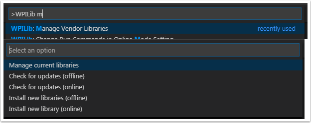
To add a vendor library that has been installed by an offline installer, press Ctrl+Shift+P and type WPILib or click on the WPILib icon in the top right to open the WPILib Command Palette and begin typing Manage Vendor Libraries, then select it from the menu. Select the option to Install new libraries (offline).
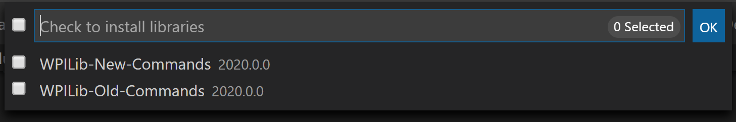
Select the desired libraries to add to the project by checking the box next to each, then click OK. The JSON file will be copied to the vendordeps folder in the project, adding the library as a dependency to the project.
Command-line
Adding a vendor library dependency from the vendor URL can also be done through the command-line via a gradle task. Open a command-line instance at the project root, and enter gradlew vendordep --url=<url> where <url> is the vendor JSON URL. This will add the vendor library dependency JSON file to the vendordeps folder of the project. Vendor libraries can be updated the same way.
The vendordep gradle task can also fetch vendordep JSONs from the user wpilib folder. To do so, pass FRCLOCAL/Filename.json as the file URL. For example, gradlew vendordep --url=FRCLOCAL/WPILibNewCommands.json will fetch the JSON for the new command-based framework.
Checking for Updates (Offline)
Dependencies are now version managed and done on a per-project bases. Even if you have installed an updated library using an offline installer, you will need to Manage Vendor Libraries and select Check for updates (offline) for each project you wish to update.
Checking for Updates (Online)
Part of the JSON file that vendors may optionally populate is an online update location. If a library has an appropriate location specified, running Check for updates (online) will check if a newer version of the library is available from the remote location.
Removing a Library Dependency
To remove a library dependency from a project, select Manage Current Libraries from the Manage Vendor Libraries menu, check the box for any libraries to uninstall and click OK. These libraries will be removed as dependencies from the project.
Libraries
Warning
These are not links to directly plug in to the VS Code -> Install New Libraries (online) feature. Click these links to visit the vendor site to see whether they offer online installers, offline installers, or both.
Copperforge LibCu Software Library - Library for all Copperforge devices including the Lasershark
CTRE Phoenix Framework - Contains CANcoder, CANifier, Pigeon IMU, Talon FX, Talon SRX, and Victor SPX Libraries and Phoenix Tuner program for configuring CTRE CAN devices
Digilent - DMC-60C library
Playing With Fusion Driver - Library for all PWF devices including the Venom motor/controller
Kauai Labs - Libraries for NavX-MXP, NavX-Micro, and Sensor Fusion
REV Robotics REVLib - Library for all REV devices including SPARK MAX and Color Sensor V3
Community Libraries
PhotonVision - Library for PhotonVision CV software
WPILib Command Libraries
Note
The project template for the Old Command Library has been removed. New projects are no longer able to be created for this, and users are highly recommended to migrate to the new library.
The WPILib old and new command libraries have been split into vendor libraries in order to reduce the chances of mixing the two which will not work correctly. They are both installed by the wpilib installer for offline installation. They may also be installed with the following online links:
Old Command Library New Command Library
To remove a library dependency from a project, select Manage Current Libraries from the Manage Vendor Libraries menu, check the box for any libraries to uninstall and click OK. These libraries will be removed as dependencies from the project.
Romi Library
A Romi Library has been created to contain several helper classes that are a part of the RomiReference example.
Building and Deploying Robot Code
Robot projects must be compiled (“built”) and deployed in order to run on the roboRIO. Since the code is not compiled natively on the robot controller, this is known as “cross-compilation.”
To build and deploy a robot project, do one of:
Open the Command Palette and enter/select “Build Robot Code”
Open the shortcut menu indicated by the ellipses in the top right corner of the VS Code window and select “Build Robot Code”
Right-click on the build.gradle file in the project hierarchy and select “Build Robot Code”
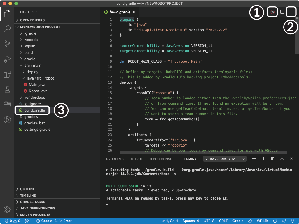
Deploy robot code by selecting “Deploy Robot Code” from any of the three locations from the previous instructions. That will build (if necessary) and deploy the robot program to the roboRIO. If successful, we will see a “Build Successful” message (1) and the RioLog will open with the console output from the robot program as it runs (2).
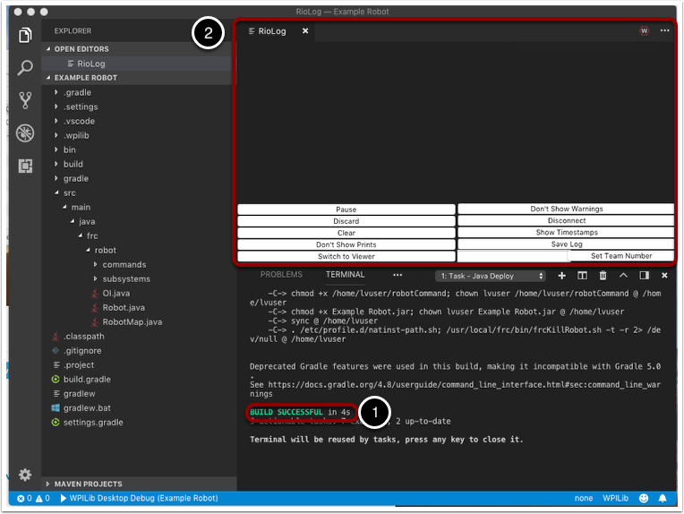
Viewing Console Output
For viewing the console output of text based programs the roboRIO implements a NetConsole. There are two main ways to view the NetConsole output from the roboRIO: The Console Viewer in the FRC Driver Station and the Riolog plugin in VS Code.
Note
On the roboRIO, the NetConsole is only for program output. If you want to interact with the system console you will need to use SSH or the Serial console.
Console Viewer
Opening the Console Viewer
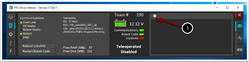
To open Console Viewer, first open the FRC® Driver Station. Then, click on the gear at the top of the message viewer window (1) and select “View Console”.
Console Viewer Window
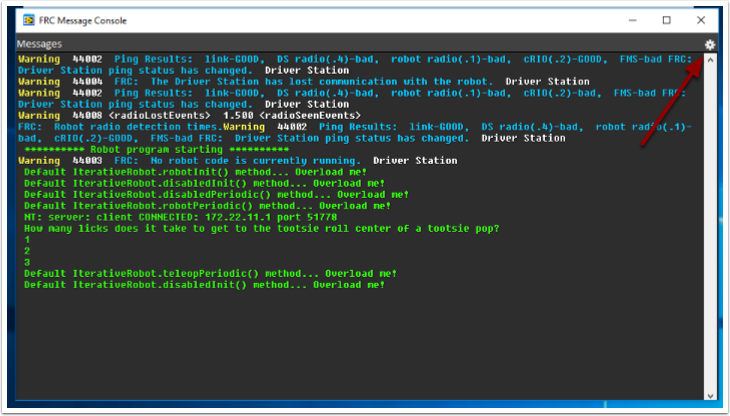
The Console Viewer window displays the output from our robot program in green. The gear in the top right can clear the window and set the level of messages displayed.
Riolog VS Code Plugin
The Riolog plugin is a VS Code view that can be used to view the NetConsole output in VS Code (credit for the original Eclipse version: Manuel Stoeckl, FRC1511).
Opening the RioLog View
By default, the RioLog view will open automatically at the end of each roboRIO deploy. To launch the RioLog view manually, press Ctrl+Shift+P to open the command palette and start typing “RioLog”, then select the WPILib: Start RioLog option.
Riolog Window
The RioLog view should appear in the top pane. The Riolog contains a number of controls for manipulating the console:
Pause/Resume Display - This will pause/resume the display. In the background, the new packets will still be received and will be displayed when the resume button is clicked.
Discard/Accept Incoming - This will toggle whether to accept new packets. When packets are being discarded the display will be paused and all packets received will be discarded. Clicking the button again will resume receiving packets.
Clear - This will clear the current contents of the display.
Don’t Show/Show Prints - This shows or hides messages categorized as print statements
Switch to Viewer - This switches to viewer for saved log files
Don’t Show/Show Warnings - This shows or hides messages categorized as warnings
Disconnect/Reconnect - This disconnects or reconnects to the console stream
Show/Don’t Show Timestamps - Shows or hides timestamps on messages in the window
Save Log - Copies the log contents into a file you can save and view or open later with the RioLog viewer (see Switch to Viewer above)
Set Team Number - Sets the team number of the roboRIO to connect to the console stream on, set automatically if RioLog is launched by the deploy process
Debugging a Robot Program
Inevitably, a program will not behave in the way we expect it to behave. When this occurs, it becomes necessary to figure out why the program is doing what it is doing, so that we can make it do what we want it to do, instead. Such an undesired program behavior is called a “bug,” and this process is called “debugging.”
A debugger is a tool used to control program flow and monitor variables in order to assist in debugging a program. This section will describe how to set up a debug session for an FRC® robot program.
Note
For beginning users who need to debug their programs but do not know/have time to learn how to use a debugger, it is often possible to debug a program simply by printing the relevant program state to the console. However, it is strongly recommended that students eventually learn to use a debugger.
Running the Debugger
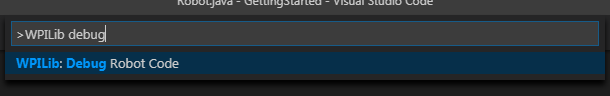
Press Ctrl+Shift+P and type WPILib or click on the WPILib Menu Item to open the Command palette with WPILib pre-populated. Type Debug and select the Debug Robot Code menu item to start debugging. The code will download to the roboRIO and begin debugging.
Breakpoints
A “breakpoint” is a line of code at which the debugger will pause the program execution so that the user can examine the program state. This is extremely useful while debugging, as it allows the user to pause the program at specific points in problematic code to determine where exactly the program is deviating from the expected behavior.
The debugger will automatically pause at the first breakpoint it encounters.
Setting a Breakpoint
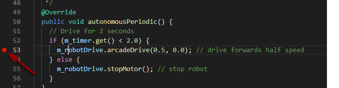
Click in the left margin of the source code window (to the left of the line number) to set a breakpoint in your user program: A small red circle indicates the breakpoint has been set on the corresponding line.
Debugging with Print Statements
Another way to debug your program is to use print statements in your code and view them using the RioLog in Visual Studio Code or the Driver Station. Print statements should be added with care as they are not very efficient especially when used in high quantities. They should be removed for competition as they can cause loop overruns.
System.out.print("example");
wpi::outs() << "example\n";
Debugging with NetworkTables
NetworkTables can be used to share robot information with your debugging computer. NetworkTables can be viewed with your favorite Dashboard or OutlineViewer. One advantage of NetworkTables is that tools like Shuffleboard can be used to graphically analyze the data. These same tools can then be used with same data to later provide an operator interface for your drivers.
Learn More
To learn more about debugging with VS Code see this link.
Some of the features mentioned in this VS Code article will help you understand and diagnose problems with your code. The Quick Fix (yellow light bulb) feature can be very helpful with a variety of problems including what to import.
One of the best ways to prevent having to debug so many issues is to do Unit Testing.
Verifying that your robot works in Simulation is also a great way to prevent having to do complex debugging on the actual robot.
Importing a Gradle Project
Due to changes in the project, it is necessary to update the build files for a previous years Gradle project. It is also necessary to import vendor libraries again, since last year’s vendor libraries must be updated to be compatible with this year’s projects.
Automatic Import
To make it easy for teams to import previous years gradle projects into the current year’s framework, WPILib includes a wizard for importing previous years projects into VS Code. This will generate the necessary gradle components and load the project into VS Code. In place upgrades are not supported. The importer automatically imports the old or new command framework 3rd party library (which ever one was used on the imported project).
Important
The import process copies your project source files from the current directory to a new directory and completely regenerates the gradle files. Additionally, it updates the code for the package changes made in 2022. If you made non-standard updates to the build.gradle, you will need to make those changes again. For this reason, in place upgrades are not supported. It is also necessary to import vendor libraries again, since last year’s vendor libraries must be updated to be compatible with this year’s projects.
Launching the Import Wizard
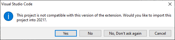
When you open a previous year’s project, you will be prompted to import that project. Click yes.
Alternately, you can chose to import it from the menu. Press Ctrl+Shift+P and type “WPILib” or click the WPILib icon to locate the WPILib commands. Begin typing “Import a WPILib 2020/2021 Gradle project” and select it from the dropdown as shown below.
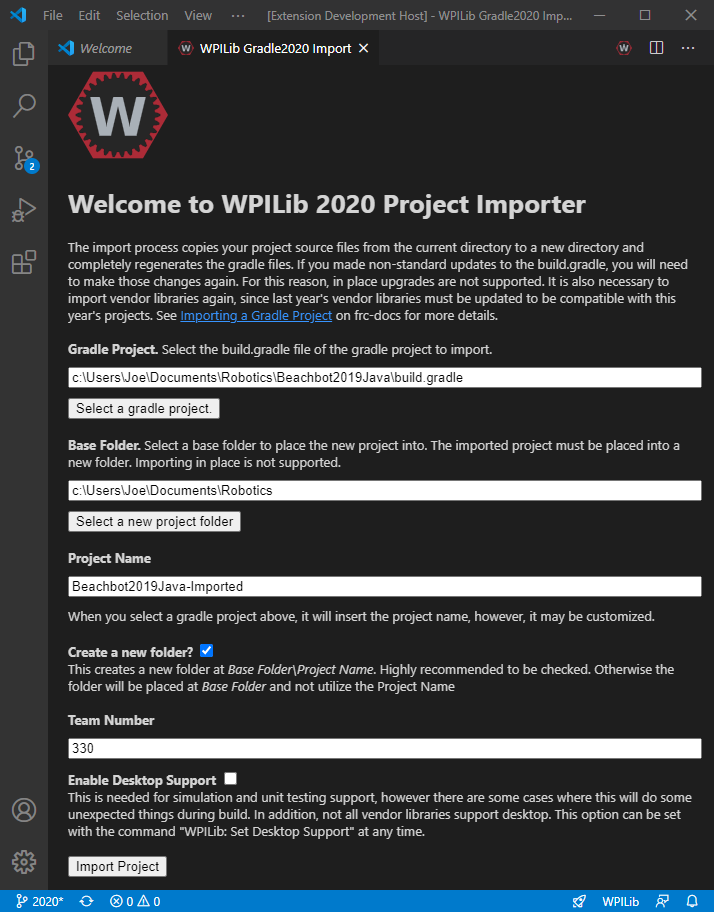
You’ll be presented with the WPILib Project Importer window. This is similar to the process of creating a new project and the window and the steps are shown below. This window contains the following elements:
Gradle Project: Selects the project to be imported. Users should select the build.gradle file in the root directory of the gradle project.
Project Location: This determines the folder in which the robot project will be located.
Project Name: The name of the robot project. This also specifies the name that the project folder will be given if the Create New Folder box is checked. This must be a different directory from the original location.
Create a New Folder: If this is checked, a new folder will be created to hold the project within the previously-specified folder. If it is not checked, the project will be located directly in the previously-specified folder. An error will be thrown if the folder is not empty and this is not checked.
Team Number: The team number for the project, which will be used for package names within the project and to locate the robot when deploying code.
Enable Desktop Support: If this is checked, simulation and unit test support is enabled. However, there are some cases where this will do some unexpected things. In addition, all vendor libraries need desktop support which not all libraries do.
Click Import Project to begin the upgrade.
The gradle project will be upgraded and copied into the new project directory. You can then either open the new project immediately using the pop-up below or open it later using the Ctrl+O (or Command+O for macOS) shortcut.
Click Yes I trust the authors.
C++ Configurations (C++ Only)
For C++ projects, there is one more step to set up IntelliSense. Whenever you open a project, you should get a pop-up in the bottom right corner asking to refresh C++ configurations. Click Yes to set up IntelliSense.
3rd Party Libraries
It is necessary to update and re-import 3rd party libraries. See 3rd Party Libraries for details.
Using Test Mode
Test mode is designed to enable programmers to have a place to put code to verify that all systems on the robot are functioning. In each of the robot program templates there is a place to add test code to the robot. If you use the TimedRobot template, or use command-based programming you can easily see the operation of all the motors and sensors through the LiveWindow.
Enabling Test Mode
Test mode on the robot can be enabled from the Driver Station just like autonomous or teleop. When in test mode, the testInit method is run once, and the testPeriodic method is run once per tick, in addition to robotPeriodic, the same as teleop and autonomous control modes. To enable test mode in the Driver Station, select the “Test” button and enable the robot. The test mode code will then run.
Adding Test mode code to your robot code
Adding test mode can be as painless as calling your already written Teleop methods from Test. This will allow you to use the LiveWindow tuning features for classes such as PIDBase and PIDController, as well as PIDSubsystems and PIDCommands, to change PID constants and setpoints. Make sure to add your subsystems to SmartDashboard with the putData(subsystem) or PutData(subsystem) method.
public class Robot extends TimedRobot {

    @Override
    public void robotInit() {
        SmartDashboard.putData(m_aSubsystem);
    }

    @Override
    public void testInit() {
        teleopInit();
    }

    @Override
    public void testPeriodic() {
        teleopPeriodic();
    }
}
void Robot::RobotInit() {
    SmartDashboard::PutData(m_aSubsystem);
}

void Robot::TestInit() {
    TestInit();
}

void Robot::TestPeriodic() {
    TeleopPeriodic();
}
Test Mode in SmartDashboard
The above sample code produces the following output when the Driver Station is put into Test mode then enabled. You can operate the motors by moving the sliders and read the values of sensors such as the wrist potentiometer.
Notice that the values are grouped by the subsystem names to group related actuators and sensors for easy testing. The subsystem names are specified by supplying a name to the putData() method, or by calling SendableRegistry.setName(). This grouping, while not required, makes it much easier to test one subsystem at a time and have all the values next to each other on the screen.
Using Test Mode with the TimedRobot Template
The TimedRobot template lends itself quite nicely to testing since it will periodically call the testPeriodic() method (or TestPeriodic() in C++) in your robot program. The testPeriodic() method will be called every 20ms and it is a good place to test commands or have LiveWindow update. The LiveWindow updating is built into the TimedRobot template so there is very little work to use LiveWindow.
Note
This works even if you are using the TimedRobot template and not doing Command-based programming.
In this example the sensors are registered with the LiveWindow and during the testPeriodic method, simply update all the values by calling the LiveWindow run() method. If your program is causing too much network traffic you can call the run method less frequently by, for example, only calling it every 5 updates for a 100ms update rate.
PID Tuning in Test Mode
Tuning PID loops is often a challenging prospect with frequent recompiles of the program to get the correct values. When using the command based programming model, subclassing PIDSubsystem or PIDCommand in your PID commands allows the adjustment of PID constants with immediate feedback of the results.
Dashboards
Shuffleboard
Shuffleboard - Getting Started
Tour of Shuffleboard
Shuffleboard is a dashboard for FRC® based on newer technologies such as JavaFX that are available to Java programs. It is designed to be used for creating dashboards for C++ and Java programs. If you’ve used SmartDashboard in the past then you are already familiar with many of the features of Shuffleboard since they fundamentally work the same way. But Shuffleboard has many features that aren’t in SmartDashboard. Here are some of the highlights:
Graphics is based on JavaFX, the Java graphics standard. Each of the components has an associated style sheet so it becomes possible to have different “skins” or “themes” for Shuffleboard. We supply default light and dark themes.
Shuffleboard supports multiple sheets for the display of your data. In fact you can create a new sheet (shown as a tab in the Shuffleboard window) and indicate if and which data should be autopopulated on it. By default there is a Test tab and a SmartDashboard tab that are autopopulated as data arrives. Other tabs might be for robot debugging vs. driving.
Graphical display elements (widgets) are laid out on a grid to keep the interface clean and easy to read. You can change the grid size to have more or less resolution in your layouts and visual cues are provided to help you change your layout using drag and drop. Or you can choose to turn off the grid lines although the grid layout is preserved.
Layouts are saved and the previous layout is instantiated by default when you run shuffleboard again.
There is a record and playback feature that lets you review the data sent by your robot program after it finishes. That way you can carefully review the actions of the robot if something goes wrong.
Graph widgets are available for numeric data and you can drag data onto a graph to see multiple points at the same time and on the same scale.
You can extend Shuffleboard by writing your own widgets that are specific to your team’s requirements. Documentation on extending it are on the Shuffleboard GitHub Wiki.
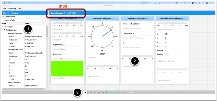
Sources area: Here are data sources from which you can choose values from NetworkTables or other sources to display by dragging a value into one of the tabs
Tab panes: This is where you data is displayed from the robot or other sources. In this example it is Test-mode subsystems that are shown here in the LiveWindow tab. This area can show any number of tabbed windows, and each window has it’s own set of properties like grid size and auto-populate.
Record/playback controls: set of media-like controls where you can playback the current session to see historical data
Starting Shuffleboard
You can start Shuffleboard in one of four ways:
You can automatically start it when the Driver Station starts by setting the “Dashboard Type” to Shuffleboard in the settings tab as shown in the picture above.
You can run it by double-clicking the Shuffleboard icon in the WPILib tools folder on the Windows Desktop.
You can run it by double-clicking on the shuffleboard.XXX file (where XXX is
.vbson Windows and.pyon Linux or macOS) in~/WPILib/YYYY/tools/(where YYYY is the year and ~ isC:\Users\Publicon Windows). This is useful on a development system that does not have the Driver Station installed such as a macOS or Linux system.You can start it from the command line by typing the command:
shuffleboardon Windows orpython shuffleboard.pyon macOS or Linux from~/WPILib/YYYY/toolsdirectory (where YYYY is the year and ~ isC:\Users\Publicon Windows). This is often easiest on a a development system that doesn’t have the Driver Station installed.
Note
The .vbs (Windows) and .py (macOS/Linux) scripts help launch the tools using the correct JDK.
Getting robot data onto the dashboard
The easiest way to get data displayed on the dashboard is simply to use methods in the SmartDashboard class. For example to write a number to Shuffleboard write:
SmartDashboard.putNumber("Joystick X value", joystick1.getX());
to see a field displayed with the label “Joystick X value” and a value of the X value of the joystick. Each time this line of code is executed, a new joystick value will be sent to Shuffleboard. Remember: you must write the joystick value whenever you want to see an updated value. Executing this line once at the start of the program will only display the value once at the time the line of code was executed.
Displaying data from your robot
Your robot can display data in regular operating modes like Teleop and Autonomous modes but you can also display the status and operate all the robot subsystems when the robot is switched to Test mode. By default you’ll see two tabs when you start Shuffleboard, one for Teleop/Autonomous and another for Test mode. The currently selected tab is underlined as can be seen in the picture below.
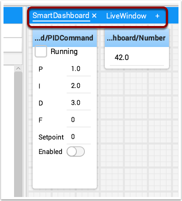
Often debugging or monitoring the status of a robot involves writing a number of values to the console and watching them stream by. With Shuffleboard you can put values to a GUI that is automatically constructed based on your program. As values are updated, the corresponding GUI element changes value - there is no need to try to catch numbers streaming by on the screen.
Displaying values in normal operating mode (autonomous or teleop)
protected void execute() {
    SmartDashboard.putBoolean("Bridge Limit", bridgeTipper.atBridge());
    SmartDashboard.putNumber("Bridge Angle", bridgeTipper.getPosition());
    SmartDashboard.putNumber("Swerve Angle", drivetrain.getSwerveAngle());
    SmartDashboard.putNumber("Left Drive Encoder", drivetrain.getLeftEncoder());
    SmartDashboard.putNumber("Right Drive Encoder", drivetrain.getRightEncoder());
    SmartDashboard.putNumber("Turret Pot", turret.getCurrentAngle());
    SmartDashboard.putNumber("Turret Pot Voltage", turret.getAverageVoltage());
    SmartDashboard.putNumber("RPM", shooter.getRPM());
}
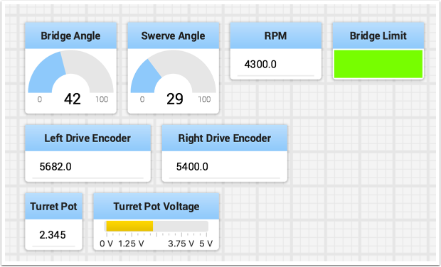
You can write Boolean, Numeric, or String values to Shuffleboard by simply calling the correct method for the type and including the name and the value of the data, no additional code is required.
Numeric types such as char, int, long, float or double call SmartDashboard.putNumber(“dashboard-name”, value).
String types call SmartDashboard.putString(“dashboard-name”, value)
Boolean types call SmartDashboard.putBoolean(“dashboard-name”, value)
Changing the display type of data
Depending on the data type of the values being sent to Shuffleboard you can often change the display format. In the previous example you can see that number values were displayed as either decimal numbers, a dial to better represent angles, and as a voltage view for the turret potentiometer. To set the display type right-click on the tile and select “Show as…”. You can choose display types from the list in the popup menu.
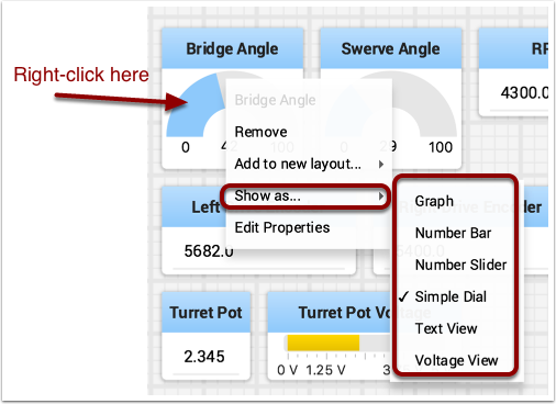
Displaying data in Test mode
You may add code to your program to display values for your sensors and actuators while the robot is in Test mode. This can be selected from the Driver Station whenever the robot is not on the field. The code to display these values is automatically generated by RobotBuilder or manually added to your program and is described in the next article. Test mode is designed to verify the correct operation of the sensors and actuators on a robot. In addition it can be used for obtaining setpoints from sensors such as potentiometers and for tuning PID loops in your code.
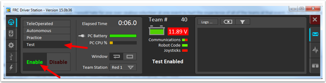
Enable Test Mode in the Driver Station by clicking on the “Test” button and setting “Enable” on the robot. When doing this, Shuffleboard will display the status of any actuators and sensors used by your program organized by subsystem.
Getting data from the Sources view
Normally NetworkTables data automatically appears on one of the tabs and you just rearrange and use that data. Sometimes you might want to recover a value that was accidentally deleted from the tab or display a value that is not part of the SmartDashboard / NetworkTables key. For these cases the values can be dragged onto a pane from NetworkTables view under Sources on the left side of the window. Choose the value that you want to display and just drag it to the pane and it will be automatically created with the default type of widget for the data type.
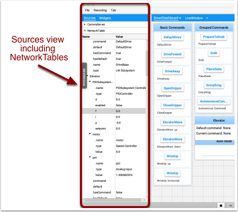
Note
Sometimes the Sources view is not visible on the left - it is possible to drag the divider between the tabbed panes and the Sources so the sources is not visible. If this happens move the cursor over the left edge and look for a divider resizing cursor, then left click and drag out the view. In the two images below you can see where to click and drag, and when finished the divider is as shown in the second image.
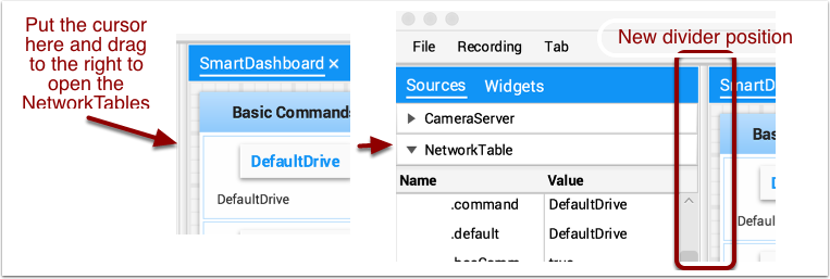
Displaying Camera Streams
Camera streams from the robot can be viewed on a tab in Shuffleboard. This is useful for viewing what the robot is seeing to give a less obstructed view for operators or helping visualize the output from a vision algorithm running on the driver station computer or a coprocessor on the robot. Any stream that is running using the CameraServer API can be viewed in a camera stream widget.
Adding a Camera Stream
To add a camera to your dashboard select “Sources” and view the “CameraServer” source in the left side panel in the Shuffleboard window as shown in the example below. A list of camera streams will be shown, in this case there is only one camera called “Robot Front Camera”. Drag that to the tab where it should be displayed. Alternatively the stream can also be placed on the dashboard by right-clicking on the stream in the Sources list and selecting “Show as: Camera Stream”.
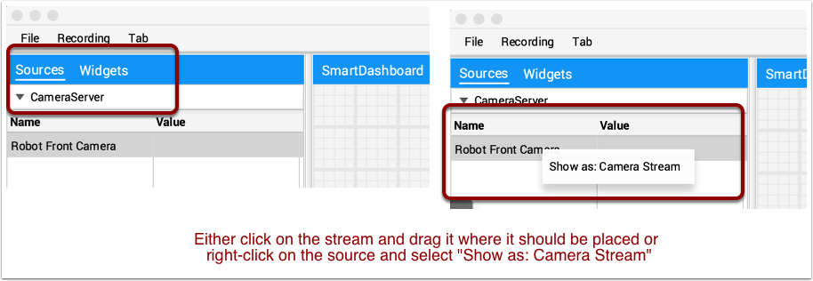
Once the camera stream is added it will be displayed in the window. It can be resized and moved where you would like it.
Note
Be aware that sending too much data from too high a resolution or too high a frame rate will cause high CPU usage on both the roboRIO and the laptop.
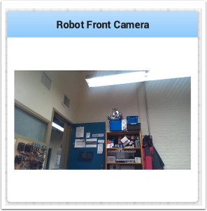
Working with widgets
The visual displays that you manipulate on the screen in Shuffleboard are called widgets. Widgets are generally automatically displayed from values that the robot program publishes with NetworkTables.
Moving widgets
Widgets can be moved simply with drag and drop. Just move the cursor over the widget, left-click and drag it to the new position. When dragging you can only place widgets on grid squares and the size of the grid will effect the resolution of your display. When dragging a red or green outline will be displayed. Green generally means that there is enough room at the current location to drop the widget and red generally means that it will overlap or be too big to drop. In the example below a widget is being moved to a location where it doesn’t fit.
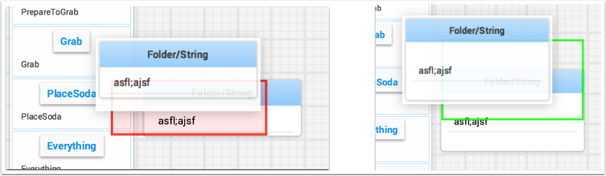
Resizing widgets
Widgets can be resized by clicking and dragging the edge or corner of the widget image. The cursor will change to a resize-cursor when it is in the right position to resize the widget. As with moving widgets, a green or red outline will be drawn indicating that the widget can be resized or not. The example below shows a widget being resized to a larger area with the green outline indicating that there is no overlap with surrounding widgets.
Changing the display type of widgets
Shuffleboard is very rich in display types depending on the data published from the robot. It will automatically choose a default display type, but you might want to change it depending on the application. To see what the possible displays are for any widget, right-click on the widget and select the “Show as…” and from the popup menu, choose the desired type. In the example below are two data values, one a number and the other a boolean. You can see the different types of display options that are available to each. The boolean value has only two possible values (true/false) it can be shown as a boolean box (the red/green color), or text, or a toggle button or toggle switch. The. number value can be displayed as a graph, number bar, number slider, dial, text, or a voltage view depending on the context of the value.
Changing the title of widgets
You can change the title of widgets by double-clicking in their title bar and editing the title to the new value. If a widget is contained in a layout, then right-click on the widget and select the properties. From there you can change the widget title that is displayed.
Changing widget properties
You can change the appearance of a widget such as the range of values represented, colors or some other visual element. In cases where this is possible right-click on the widget and select “Edit properties” from the popup menu. In this boolean value widget shown below, the widget title, true color and false color can all be edited.
Working with Lists
Lists are sets of tiles that are be logically grouped together in a vertical layout. When tiles are added to a list,it becomes visually obvious that the tiles are related in function. In addition tiles in lists take up less screen space than the same tiles directly on the desktop because tiles in a list don’t display the dark window title, but instead display a smaller textual label documenting the contents of the list.
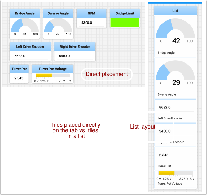
Creating a list
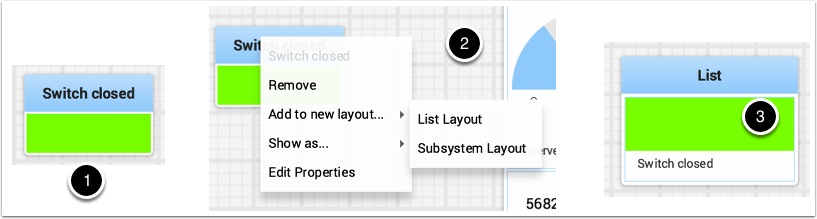
A list can be created by: 1. Right-clicking on the first tile that should go into the list. 2. Select the “Add to new layout…” option from the popup menu. 3. A new list will be created called “List” and the tile will be at the top of it. Notice that tiles in lists do not have the window title at the top, but instead have the text that was in the window title.
Adding tiles to a list
Add tiles to a list layout by: 1. identify the list and the tile to be added. 2. Drag the new tile onto the list. 3. The tile will be added to the list. If there is no room as the list is currently sized, the tile will be added off the end of the list and a vertical scrollbar will be added if it’s not already there.
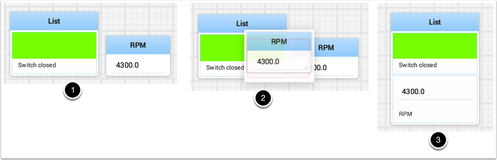
Rearranging tiles in a list
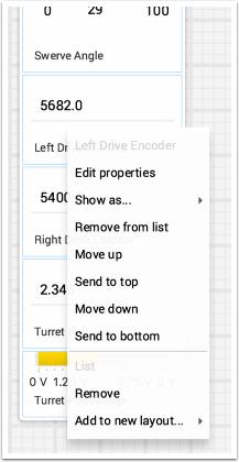
Tiles in a list can be rearranged by right-clicking on the tile to be moved and selecting:
“Move up” to move the tile before the previous tile
“Move down” to move the tile after the next tile
“Send to top” to move the tile to the top of the list
“Send to bottom” to move the tile to the bottom of the list
“Remove from list” to delete the tile from the list.
Renaming a list
You can rename a list by double-clicking on the list title and changing the name. Click outside fo the title to save the changes
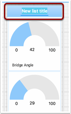
Creating and manipulating tabs
The tabbed layout the Shuffleboard uses help separate different “views” of your robot data and make the displays more useful. You might have a tab the has the display for helping debug the robot program and a different tab for use in competitions. There are a number of options that make tabs very powerful. You can control which data from NetworkTables or other sources appears in each of your tabs using the auto-populate options described later in this article.
Default tabs
When you open Shuffleboard for the first time there are two tabs, labeled SmartDashboard and LiveWindow. These correspond to the two views that SmartDashboard had depending on whether your robot is running in Autonomous/Teleop or Test mode. In shuffleboard both of these views are available any time.
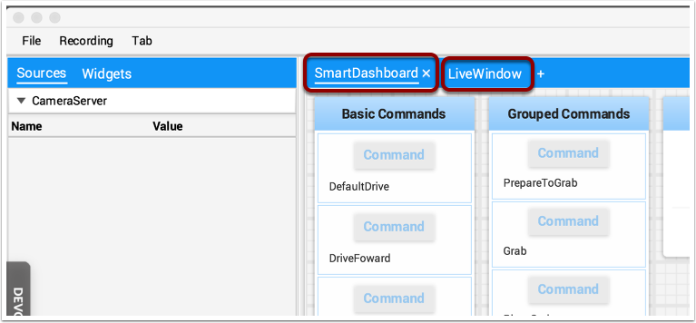
On the SmartDashboard tab all the values that are written using the SmartDashboard.putType() set of methods. On the LiveWindow tab all the autogenerated debugging values are shown.
Switching between tabs
You can switch between tabs clicking on the tab label at the top of the window. In the case above, simply click on SmartDashboard or LiveWindow to see the values that are associated with each tab.
Adding and Hiding Tabs
You can add additional tabs by clicking on the plus(+) symbol just to the right of the last tab. Once you create a new tab you can set the label by double-clicking on the label in the tab and editing it. You can also right-click on the tab or use the Tab menu to bring up the tab preferences and from that window you can change the name by editing the Title field.
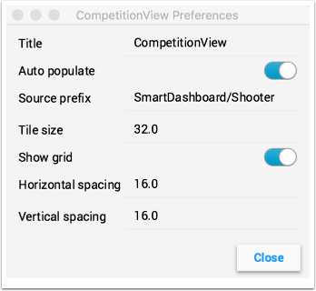
You can hide tabs by clicking the minus(-) symbol to the left of the selected tab name. Since tabs are generated based on the relevant NetworkTable, it is not possible to permanently delete them without deleting the table.
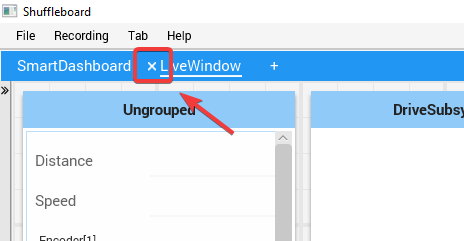
Setting the tab to auto-populate
One of the most powerful features with tabs is to have them automatically populate new values based on a source prefix that is supplied in the tab Preferences pane. In the above example the Preferences pane has a Source prefix of “SmartDashboard/Shooter” and Auto populate is turned on. Any values that are written using the SmartDashboard class that specifies a sub-key of Shooter will automatically appear on that tab. Note: keys that match more than one Source prefix will appear in both tabs. Because those keys also start with SmartDashboard/ and that’s the Source prefix for the default SmartDashboard tab, those widgets will appear in both panes. To only have values appear in one pane, you can use NetworkTables to write labels and values and use a different path that is not under SmartDashboard. Alternatively you could let everything appear in the SmartDashboard tab making it very cluttered, but have specific tabs for your needs that will be better filtered.
Using the tab grid and spacing
Each tab can have it’s own Tile size (number of pixels per large square). So some tabs might have coarser resolution for easier layout and others might have a fine grid. The Tile size in the Tab preferences overrides any global settings in the Shuffleboard preferences. In addition, you can specify the padding between the drawing in the widget and the edge of the of the widget. If you program user interfaces these parameters are usually referred to as horizontal and vertical gap (hgap, vgap).
Moving widgets between tabs
Currently there is no way to easily move widgets between tabs without deleting it from one tab and dragging the field from the sources hierarchy on the left into the new pane. We hope to have that capability in a subsequent update soon.
Working with Graphs
With Shuffleboard you can graph numeric values over time. Graphs are very. useful to see how sensor or motor values are changing as your robot is operating. For example the sensor value can be graphed in a PID loop to see how it is responding during tuning.
To create a graph, choose a numeric value and right-click in the heading and select “Show as…” and then choose graph
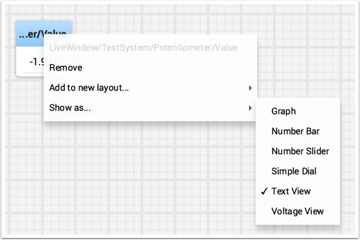
The graph widget shows line plots of the value that you selected. It will automatically set the scale and the default time interval that the graph will show will be 30 seconds. You can change that in the setting for the graph (see below).
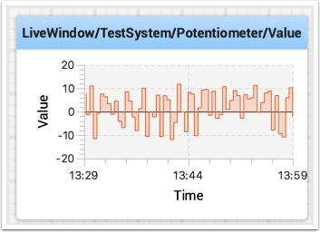
Adding Additional Data Values
For related values it is often desirable to show multiple values on the same graph. To do that, simply drag additional values from the NetworkTables source view (left side of the Shuffleboard window) and drop it onto the graph and that value will be added as shown below. You can continue to drag additional values onto the graph.
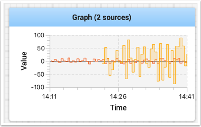
You can resize the graph vertically to view the legend if it is not displayed as shown in the image below. The legend shows all the sources that are used in the plot.
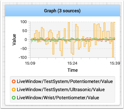
Setting Graph Properties
You can set the number of seconds that are shown in the graph by changing the “Visible time” in the graph widget properties. To access the properties, right-click on the graph and select “Edit properties”.
In addition to setting the visible time the graph can selectively turn sources on and off by turning the switch on and off for each of the sources shown in the properties window (see below).
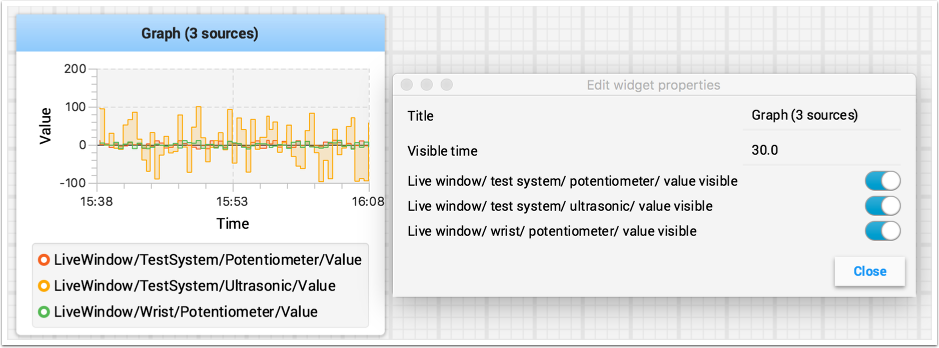
Recording and Playback
Shuffleboard can log all widget updates during a session. Later the log file can be “played back” to see what happened during a match or a practice run. This is especially useful if something doesn’t operate as intended during a match and you want to see what happened. Each recording is captured in a recording file.
Creating a Recording
When shuffleboard starts it begins recording to all the NetworkTables values are recorded and continues until stopped by hitting the record/stop button in the recorder controls as shown below. If a new recording is desired, such as when a new piece of code or mechanical system is being tested, stop the current recording if it is running, and click the record button. Click the button again to stop recording and close the recording file. If the button is round (as shown) then click it to start a recording. If the button is a square, then a recoding is currently running so click it to stop the recording.
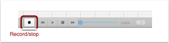
Playing a Recording
Previous recordings can be played back by:
Selecting the “Recording” menu then click “Load playback”.
Choose a recording from the from the directory shown. Recordings are grouped by date and the file names are the time the recording was made to help identify the correct one. Select the correct recording from the list.
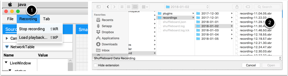
Controlling the Playback
Selecting the recoding file will begin playback of that file. While the recording is playing the recording controls will show the current time within the recording as well as the option to loop the recording while watching it. When the recording is being played back the “transport” controls will allow the playback to be controlled.
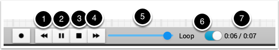
The controls work as follows:
The left double-arrow button backs up the playback to the last changed data point
The play/pause controls starts and stops the playback
The square stop button stops playback and resumes showing current robot values
The right double-arrow skips forward to the next changed data value
The slider allows for direct positioning to any point in time to view different parts of the recording
The loop switch turns on playback looping, that is, the playback will run over and over until stopped
The time shows the current point within the recording and the total time of the recording
Converting to Different File Formats
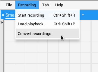
Shuffleboard recordings are in a custom binary format for efficiency. To analyze recorded data without playing it back through the app, Shuffleboard supports data converters to convert the recordings to an arbitrary format. Only a simple CSV converter is shipped with the app, but teams can write custom converters and include them in Shuffleboard plugins.
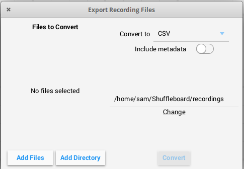
Multiple recordings can be converted at once. Individual files can be selected with the “Add Files” button, or all recording files in a directory can be selected at once with the “Add Directory” button.
Converted recordings will be generated in the ~/Shuffleboard/recordings directory, but can be manually selected with the “Change” button.
Different converters can be selected with the dropdown in the top right. By default, only the CSV converter is available. Custom converters from plugins will appear as options in the dropdown.
Additional Notes
Graphs won’t display properly while scrubbing the timeline but if it is playing through where the graph history can be captured by the graph then they will display as in the original run.
Setting global preferences for Shuffleboard
There are a number of settings that set the way Shuffleboard looks and behaves. Those are on the Shuffleboard Preferences pane that can be accessed from the File menu.
Setting the theme
Shuffleboard supports two themes, Material Dark and Material Light and the setting depends on your preferences. This uses css styles that apply to the entire application and can be changed any time.
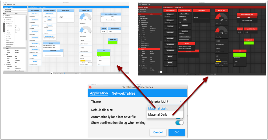
Setting the default tile size
Shuffleboard positions tiles on a grid when you are adding or moving them yourself or when they are auto-populated. You can set the default tile size when for each tab or it can be set globally for all the tabs created after the default setting is changed. Finer resolution in the grid results in finer control over placement of tiles. This can be set in the Shuffleboard Preferences window as shown below.
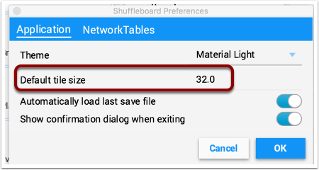
Working with the layout save files
You can save your layout using the File / Save and File / Save as… menu options. The preferences window has options to cause the previous layout to be automatically applied when Shuffleboard starts. In addition, Shuffleboard will display a “Save layout” window to remind you to save the layout on exit, if the layout has changed. You can choose to turn off the automatic prompt on exit, but be sure to save the layout manually in this case so you don’t loose your changes.
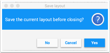
Setting the team number
In order for Shuffleboard to be able to find your NetworkTables server on your robot, specify your team number in the “NetworkTables” tab on the Preferences pane. If you’re running Shuffleboard with a running Driver Station, the Server field will be auto-populated with the correct information. If you’re running on a computer without the Driver Station, you can manually enter your team number or the robotRIO network address.
Shuffleboard FAQ, issues, and bugs
Warning
Shuffleboard as well as most of the other control system components were developed with Java 11 and will not work with Java 8. Be sure before reporting problems that your computer has Java 11 installed and is set as the default Java Environment.
Frequently Asked Questions
Bugs, issues, and feature requests can be added on the Shuffleboard GitHub page by creating an issue. We will try to address them as they are entered into the system. Please try to look at existing issues before creating new ones to make sure you aren’t duplicating something that has already been reported or work that is planned. You can find the issues on the Shuffleboard GitHub page.
The Shuffleboard wiki has a large amount of documentation on extending the program with custom plugins. In the future we will be posting a sample plugin project that can be used for additional custom widgets, but for now the wiki documentation is complete.
You can get the source code by downloading, cloning, or forking the repository on the GitHub site. To build and run Shuffleboard from the source, make sure that the current directory is the top level source code and use one of these commands:
Application |
Command (for Windows systems run the gradlew.bat file) |
|---|---|
Running Shuffleboard |
./gradlew :app:run |
Building the APIs and utility classes for plugin creation |
./gradlew :api:shadowJar |
Building the complete application jar file |
./gradlew :app:shadowJar |
Shuffleboard - Layouts with Code
Using tabs
Shuffleboard is a tabbed interface. Each tab organizes widgets in a logical grouping. By default, Shuffleboard has tabs for the legacy SmartDashboard and LiveWindow - but new tabs can now be created in Shuffleboard directly from a robot program for better organization.
Creating a new tab
ShuffleboardTab tab = Shuffleboard.getTab("Tab Title");
ShuffleboardTab& tab = Shuffleboard::GetTab("Tab Title");
Creating a new tab is as simple as calling a single method on the Shuffleboard class, which will create a new tab on Shuffleboard and return a handle for adding your data to the tab. Calling getTab multiple times with the same tab title will return the same handle each time.
Selecting a tab
Shuffleboard.selectTab("Tab Title");
Shuffleboard::SelectTab("Tab Title");
This method lets a tab be selected by title. This is case-sensitive (so “Tab Title” and “Tab title” are two individual tabs), and only works if a tab with that title exists at the time the method is called, so calling selectTab("Example")will only have an effect if a tab named “Example” has previously been defined.
This method can be used to select any tab in Shuffleboard, not just ones created by the robot program.
Caveats
Tabs created from a robot program differ in a few important ways from normal tabs created from the dashboard:
Not saved in the Shuffleboard save file
No support for autopopulation
Users are expected to specify the tab contents in their robot program
Have a special color to differentiate from normal tabs
Sending data
Unlike SmartDashboard, data cannot be sent directly to Shuffleboard without first specifying what tab the data should be placed in.
Sending simple data
Sending simple data (numbers, strings, booleans, and arrays of these) is done by calling add on a tab. This method will set the value if not already present, but will not overwrite an existing value.
Shuffleboard.getTab("Numbers")
     .add("Pi", 3.14);
Shuffleboard::GetTab("Numbers")
     .Add("Pi", 3.14);
If data needs to be updated (for example, the output of some calculation done on the robot), call getEntry() after defining the value, then update it when needed or in a periodic function
class VisionCalculator {
   private ShuffleboardTab tab = Shuffleboard.getTab("Vision");
   private NetworkTableEntry distanceEntry =
       tab.add("Distance to target", 0)
          .getEntry();

   public void calculate() {
     double distance = ...;
     distanceEntry.setDouble(distance);
   }
 }
Making choices persist between reboots
When configuring a robot from the dashboard, some settings may want to persist between robot or driverstation reboots instead of having drivers remember (or forget) to configure the settings before each match.
Simply using addPersistent instead of add will make the value saved on the roboRIO and loaded when the robot program starts.
Note
This does not apply to sendable data such as choosers or motor controllers.
Shuffleboard.getTab("Drive")
     .addPersistent("Max Speed", 1.0);
Sending sensors, motors, etc
Analogous to SmartDashboard.putData, any Sendable object (most sensors, motor controllers, and SendableChoosers) can be added to any tab
Shuffleboard.getTab("Tab Title")
     .add("Sendable Title", mySendable);
Retrieving data
Unlike SmartDashboard.getNumber and friends, retrieving data from Shuffleboard is also done through the NetworkTableEntries, which we covered in the previous article.
class DriveBase extends Subsystem {
   private ShuffleboardTab tab = Shuffleboard.getTab("Drive");
   private NetworkTableEntry maxSpeed =
       tab.add("Max Speed", 1)
          .getEntry();

   private DifferentialDrive robotDrive = ...;

   public void drive(double left, double right) {
     // Retrieve the maximum speed from the dashboard
     double max = maxSpeed.getDouble(1.0);
     robotDrive.tankDrive(left * max, right * max);
   }
}
This basic example has a glaring flaw: the maximum speed can be set on the dashboard to a value outside [0, 1] - which could cause the inputs to be saturated (always at maximum speed), or even reversed! Fortunately, there is a way to avoid this problem - covered in the next article.
Configuring widgets
Robot programs can specify exactly which widget to use to display a data point, as well as how that widget should be configured. As there are too many widgets to be listed here, consult the docs for details.
Specifying a widget
Call withWidget after add in the call chain:
Shuffleboard.getTab("Drive")
 .add("Max Speed", 1)
 .withWidget(BuiltInWidgets.kNumberSlider) // specify the widget here
 .getEntry();
In this example, we configure the “Max Speed” widget to use a slider to modify the values instead of a basic text field.
Setting widget properties
Since the maximum speed only makes sense to be a value from 0 to 1 (full stop to full speed), a slider from -1 to 1 can cause problems if the value drops below zero. Fortunately, we can modify that using the withProperties method
Shuffleboard.getTab("Drive")
    .add("Max Speed", 1)
    .withWidget(BuiltInWidgets.kNumberSlider)
    .withProperties(Map.of("min", 0, "max", 1)) // specify widget properties here
    .getEntry();
Notes
Widgets can be specified by name; however, names are case- and whitespace-sensitive (“Number Slider” is different from “Number slider” and “NumberSlider”). For this reason, it is recommended to use the built in widgets class to specify the widget instead of by raw name. However, a custom widget can only be specified by name or by creating a custom WidgetType for that widget.
Widget property names are neither case-sensitive nor whitespace-sensitive (“Max” and “max” are the same). Consult the documentation on the widget in the BuiltInWidgets class for details on the properties of that widget.
Organizing Widgets
Setting Widget Size and Position
Call withSize and withPosition to set the size and position of the widget in the tab.
withSize sets the number of columns wide and rows high the widget should be. For example, calling withSize(1, 1) makes the widget occupy a single cell in the grid. Note that some widgets have a minimum size that may be greater than the specified size, in which case the widget will use the smallest supported size.
withPosition sets the row and column of the top-left corner of the widget. Rows and columns are both 0-indexed, so the topmost row is number 0 and the leftmost column is also number 0. If the position of any widget in a tab is specified, every widget should also have its position set to avoid overlapping widgets.
Shuffleboard.getTab("Pre-round")
  .add("Auto Mode", autoModeChooser)
  .withSize(2, 1) // make the widget 2x1
  .withPosition(0, 0); // place it in the top-left corner
frc::Shuffleboard::GetTab("Pre-round")
  .Add("Auto Mode", autoModeChooser)
  .WithSize(2, 1)
  .WithPosition(0,0);
Adding Widgets to Layouts
If there are many widgets in a tab with related data, it can be useful to place them into smaller subgroups instead of loose in the tab. Much like how the handle to a tab is retrieved with Shuffleboard.getTab, a layout inside a tab (or even in another layout) can be retrieved with ShuffleboardTab.getLayout.
ShuffleboardLayout elevatorCommands = Shuffleboard.getTab("Commands")
  .getLayout("Elevator", BuiltInLayouts.kList)
  .withSize(2, 2)
  .withProperties(Map.of("Label position", "HIDDEN")); // hide labels for commands

elevatorCommands.add(new ElevatorDownCommand());
elevatorCommands.add(new ElevatorUpCommand());
// Similarly for the claw commands
wpi::StringMap<std::shared_ptr<nt::Value>> properties{
  std::make_pair("Label position", nt::Value::MakeString("HIDDEN"))
};

frc::ShuffleboardLayout& elevatorCommands = frc::Shuffleboard::GetTab("Commands")
  .GetLayout("Elevator", frc::BuiltInLayouts::kList)
  .WithSize(2, 2)
  .WithProperties(properties);

ElevatorDownCommand* elevatorDown = new ElevatorDownCommand();
ElevatorUpCommand* elevatorUp = new ElevatorUpCommand();

elevatorCommands.Add("Elevator Down", elevatorDown);
elevatorCommands.Add("Elevator Up", elevatorUp);
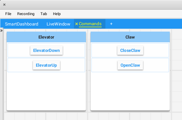
Shuffleboard - Advanced Usage
Commands and Subsystems
When using the command-based framework Shuffleboard makes it easier to understand what the robot is doing by displaying the state of various commands and subsystems in real-time.
Displaying Subsystems
To see the status of a subsystem while the robot is operating in either autonomous or teleoperated modes, that is what its default command is and what command is currently using that subsystem, send a subsystem instance to Shuffleboard:
SmartDashboard.putData(subsystem-reference);
SmartDashboard::PutData(subsystem-pointer);
Shuffleboard will display the subsystem name, the default command associated with this subsystem, and the currently running command. In this example the default command for the Elevator subsystem is called AutonomousCommand and it is also the current command that is using the Elevator subsystem.
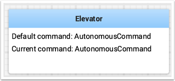
Subsystems in Test Mode
In Test mode (Test/Enabled in the driver station) subsystems may be displayed in the LiveWindow tab with the sensors and actuators of the subsystem. This is ideal for verifying of sensors are working by seeing the values that they are returning. In addition, actuators can be operated. For example, motors can be operated using sliders to set their commanded speed and direction. For PIDSubsystems the P, I, D, and F constants are displayed along with the setpoint and an enable control. This is useful for tuning PIDSubsystems by adjusting the constants, putting in a setpoint, and enabling the embedded PIDController. Then the mechanism’s response can be observed. This cycle (change parameters, enable, and observe) can be repeated until a reasonable set of parameters is found.
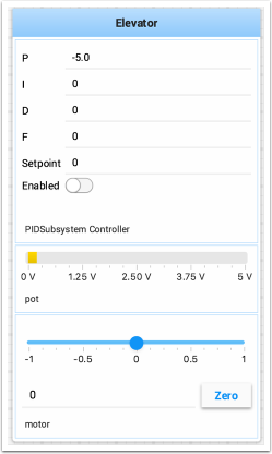
More information on tuning PIDSubsystems can be found here. Using RobotBuilder will automatically generate the code to get the subsystem displayed in Test mode. The code that is necessary to have subsystems displayed is shown below where subsystem-name is a string containing the name of the subsystem:
setName(subsystem-name);
Displaying Commands
Using commands and subsystems makes very modular robot programs that can easily be tested and modified. Part of this is because commands can be written completely independently of other commands and can therefor be easily run from Shuffleboard. To write a command to Shuffleboard use the SmartDashboard.putData method as shown here:
SmartDashboard.putData("ElevatorMove: up", new ElevatorMove(2.7));
SmartDashboard::PutData("ElevatorMove: up", new ElevatorMove(2.7));
Shuffleboard will display the command name and a button to execute the command. In this way individual commands and command groups can easily be tested without needing special test code in a robot program. In the image below there are a number of commands contained in a Shuffleboard list. Pressing the button once runs the command and pressing it again stops the command. To use this feature the robot must be enabled in teleop mode.
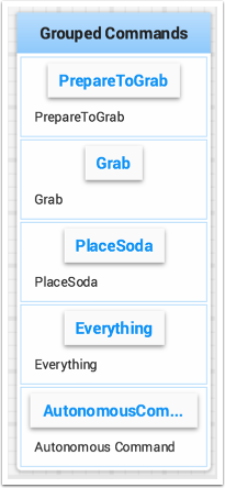
Testing and Tuning PID Loops
One challenge in using sensors to control mechanisms is to have a good algorithm to drive the motors to the proper position or speed. The most commonly used control algorithm is called PID control. There is a good set of videos (look for the robot controls playlist) that explain the control algorithms described here The PID algorithm converts sensor values into motor speeds by:
Reading sensor values to determine how far the robot or mechanism from the desired setpoint. The setpoint is the sensor value that corresponds to the expected goal. For example, a robot arm with a wrist joint should be able to move to a specified angle very quickly and stop at that angle as indicated by a sensor. A potentiometer is a sensor that can measure. rotational angle. By connecting it to an analog input, the program can get a voltage measurement that is directly proportional to the angle.
Compute an error (the difference between the sensor value and the desired value). The sign of the error value indicates which side of the setpoint the wrist is on. For example negative values might indicate that the measured wrist angle is larger than the desired wrist angle. The magnitude of the error is how far the measured wrist angle is from the actual wrist angle. If the error is zero, then the measured angle exactly matches the desired angle. The error can be used as an input to the PID algorithm to compute a motor speed.
The resultant motor speed is them used to drive the motor in the correct direction and a speed that hopefully will reach the setpoint as quickly as possible without overshooting (moving past the setpoint).
WPILib has a PIDController class that implements the PID algorithm and accepts constants that correspond to the Kp, Ki, and Kd values. The PID algorithm has three components that contribute to computing the motor speed from the error.
P (proportional) - this is a term that when multiplied by a constant (Kp) will generate a motor speed that will help move the motor in the correct direction and speed.
I (integral) - this term is the sum of successive errors. The longer the error exists the larger the integral contribution will be. It is simply a sum of all the errors over time. If the wrist isn’t quite getting to the setpoint because of a large load it is trying to move, the integral term will continue to increase (sum of the errors) until it contributes enough to the motor speed to get it to move to the setpoint. The sum of the errors is multiplied by a constant (Ki) to scale the integral term for the system.
D (differential) - this value is the rate of change of the errors. It is used to slow down the motor speed if it’s moving too fast. It’s computed by taking the difference between the current error value and the previous error value. It is also multiplied by a constant (kd) to scale it to match the rest of the system.
Tuning the PID Controller
Tuning the PID controller consists of picking constants that will give good performance. Shuffleboard helps this process by displaying the details of a PID subsystem with a user interface for setting constant values and testing how well it operates. This is displayed while the robot is operating in test mode (done by setting “Test” in the driver station).
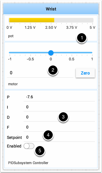
This is the test mode picture of a wrist subsystem that has a potentiometer as the sensor (pot) and a motor controller connected to the motor. It has a number of areas that correspond to the PIDSubsystem.
The analog input voltage value from the potentiometer. This is the sensor input value.
A slider that moves the wrist motor in either direction with 0 as stopped. The positive and negative values correspond to moving up or down.
The PID constants as described above (F is a feedforward value that is used for speed PID loops)
The setpoint value that corresponds the to the pot value when the wrist has reached the desired value
Enables the PID controller - No longer working, see below.
Try various PID gains to get the desired motor performance. You can look at the video linked to at the beginning of this article or other sources on the internet to get the desired performance.
Important
The enable option does not affect the PIDController introduced in 2020, as the controller is updated every robot loop. See the example below on how to retain this fuctionality.
Enable Functionality in the New PIDController
The following example demonstrates how to create a button on your dashboard that will enable/disable the PIDController.
ShuffleboardTab tab = Shuffleboard.getTab("Shooter");
NetworkTableEntry shooterEnable = tab.add("Shooter Enable", false).getEntry();

// Command Example assumed to be in a PIDSubsystem
new NetworkButton(shooterEnable).whenPressed(new InstantCommand(m_shooter::enable));

// Timed Robot Example
if (shooterEnable.getBoolean()) {
  // Calculates the output of the PID algorithm based on the sensor reading
  // and sends it to a motor
  motor.set(pid.calculate(encoder.getDistance(), setpoint));
}
frc::ShuffleboardTab& tab = frc::Shuffleboard::GetTab("Shooter");
nt::NetworkTableEntry shooterEnable = tab.Add("Shooter Enable", false).GetEntry();

// Command-based assumed to be in a PIDSubsystem
frc2::NetworkButton(shooterEnable).WhenPressed(frc2::InstantCommand([&] { m_shooter.Enable(); }));

// Timed Robot Example
if (shooterEnable.GetBoolean()) {
  // Calculates the output of the PID algorithm based on the sensor reading
  // and sends it to a motor
  motor.Set(pid.Calculate(encoder.GetDistance(), setpoint));
}
Viewing Hierarchies of Data
Dragging a key with other keys below it (deeper in the hierarchy) displays the hierarchy in a tree, similar to the NetworkTables sources on the left.
Select the data source:
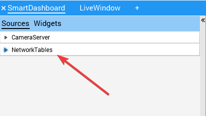
Click and drag the NetworkTables key into the preferred tab.
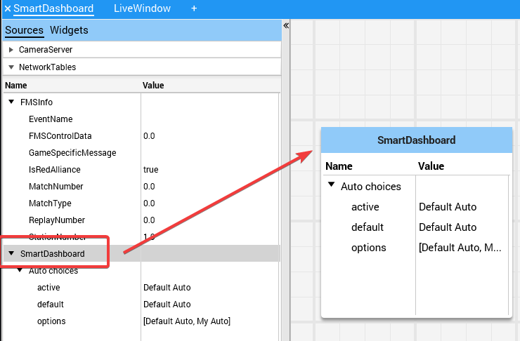
Shuffleboard - Custom Widgets
Built-in Plugins
Shuffleboard provides a number of built-in plugins that handle common tasks for FRC® use, such as camera streams, all widgets, and NetworkTables connections.
Base Plugin
The base plugin defines all the data types, widgets, and layouts necessary for FRC use. It does not define any of the source types, or any special data types or widgets for those source types. Those are handled by the NetworkTables Plugin and the CameraServer Plugin. This separation of concerns makes it easier for teams to create plugins for custom source types or protocols (eg HTTP, ZeroMQ) for the FRC data types without needing a NetworkTables client.
CameraServer Plugin
The camera server plugin provides sources and widgets for viewing camerastreams from the CameraServer WPILib class.
This plugin depends on the NetworkTables Plugin in order to discover the available camera streams.
CameraServer sources are automatically discovered by looking at the
/CameraPublisher NetworkTable.
/CameraPublisher
  /<camera name>
    streams=["url1", "url2", ...]
For example, a camera named “Camera” with a server at
roborio-0000-frc.local would have this table layout:
/CameraPublisher
  /Camera
    streams=["mjpeg:http://roborio-0000-frc.local:1181/?action=stream"]
This setup will automatically discover all camera streams hosted on a roboRIO by the CameraServer class in WPILib. Any non-WPILib projects that want to have camera streams appear in shuffleboard will have to set the streams entry for the camera server.
NetworkTables Plugin
The NetworkTables plugin provides data sources backed by ntcore. Since the LiveWindow and SmartDashboard classes in WPILib use NetworkTables to send the data to the driver station, this plugin will need to be loaded in order to use those classes.
This plugin handles the connection and reconnection to NetworkTables automatically, users of shuffleboard and writers of custom plugins will not have to worry about the intricacies of the NetworkTables protocol.
Creating a Plugin
Overview
Plugins provide the ability to create custom widgets, layouts, data sources/types, and custom themes. Shuffleboard provides the following built-in plugins.
NetworkTables Plugin: To connect to data published over NetworkTables
Base Plugin: To display custom FRC® data types in custom widgets
CameraServer Plugin: To view streams from the CameraServer
Tip
An example custom Shuffleboard plugin which creates a custom data type and a simple widget for displaying it can be found here.
Create a Custom Plugin
In order to define a plugin, the plugin class must be a subclass of edu.wpi.first.shuffleboard.api.Plugin or one of its subclasses. An example of a plugin class would be as following.
import edu.wpi.first.shuffleboard.api.plugin.Description;
import edu.wpi.first.shuffleboard.api.plugin.Plugin;

@Description(group = "com.example", name = "MyPlugin", version = "1.2.3", summary = "An example plugin")
public class MyPlugin extends Plugin {

}
Additional explanations on how these attributes are used, including version numbers can be found here.
Note the @Description annotation is needed to tell the plugin loader the properties of the custom plugin class.
Plugin classes are permitted to have a default constructor but it cannot take any arguments.
Building plugin
Plugins require the usage of the Shuffleboard API Library. These dependencies can be resolved in the build.gradle file or using maven. The dependencies would be as follows:
For Gradle:
repositories {
   mavenCentral()
   maven{ url "https://frcmaven.wpi.edu:443/artifactory/release" }
}

dependencies {
   compileOnly 'edu.wpi.first.shuffleboard:api:2020.+'
   compileOnly 'edu.wpi.first.shuffleboard.plugin:networktables:2020.+'
}
Plugins are allowed to have dependencies on other plugins and libraries, however, they must be included correctly in the maven or gradle build file. When a plugin depends on other plugins, it is good practice to define those dependencies so the plugin does not load when the dependencies do not load as well. This can be done using the @Requires annotation as shown below:
@Requires(group = "com.example", name = "Good Plugin", minVersion = "1.2.3")
@Requires(group = "edu.wpi.first.shuffleboard", "Base", minVersion = "1.0.0")
@Description(group = "com.example", name = "MyPlugin", version = "1.2.3", summary = "An example plugin")
public class MyPlugin extends Plugin {

}
The minVersion specifies the minimum allowable version of the plugin that can be loaded. For example, if the minVersion is 1.4.5, and the plugin with the version 1.4.7 is loaded, it will be allowed to do so. However, if the plugin with the version 1.2.4 is loaded, it will not be allowed to since it is less than the minVersion.
Deploying Plugin To Shuffleboard
In order to load a plugin in Shuffleboard, you will need to generate a jar file of the plugin and put it in the ~/Shuffleboard/plugins folder. This can be done automatically
from gradle as noted:
The path to your Shuffleboard plugin folder will most likely be ~/Shuffleboard/plugins.
The deployPlugin task takes four parameters, the type: Copy parameter makes the task implement the CopySpec interface
specifying what to copy. The group and description parameters to specify what the Group ID of the plugin is and a short descriptive description to what the Plugin does.
In the body, the from field specifies from where the file is to be copied from, followed by the into field specifying the destination to where the file needs to be copied to.
Finally, the include field ensures all files with the .jar extension is also copied.
After deploying, Shuffleboard will cache the path of the plugin so it can be automatically loaded the next time Shuffleboard loads. It may be necessary to click on Clear Cache under the plugins menu to remove a plugin or reload a plugin into Shuffleboard.
By running gradle deployPlugin from the command line, the jar file will automatically placed into the Shuffleboard plugin folder.
Manually Adding Plugin
The other way to add a plugin to Shuffleboard is to compile it to a jar file and add it from Shuffleboard.
First, compile your plugin into a .jar file using Maven or Gradle. Then, open Shuffleboard, click on the file tab in the top left, and choose Plugins from the drop down menu.
From the plugins window, choose the “Load plugin” button in the bottom right, and select your jar file.
Creating Custom Data Types
Widgets allow us to control and visualize different types of data. This data could be integers and doubles or even Java Objects. In order to display these types of data using widgets, it is helpful to create a container class for them. It is not necessary to create your own Data Class if the widget will handle single fielded data types such as doubles, arrays, or strings.
Creating The Data Class
In this example, we will create a custom data type for a 2D Point and its x and y coordinates. In order to create a custom data type class, it must extend the abstract class ComplexData.
Your custom data class must also implement the asMap() method that returns the represented data as a simple map as noted below with the @Override annotation:
import edu.wpi.first.shuffleboard.api.data.ComplexData;

import java.util.Map;

public class MyPoint2D extends ComplexData<MyPoint2D> {

   private final double x;
   private final double y;

   //Constructor should take all the different fields needed and assign them their corresponding instance variables.
   public MyPoint2D(double x, double y) {
      this.x = x;
      this.y = y;
   }

   @Override
   public Map<String, Object> asMap() {
      return Map.of("x", x, "y", y);
   }
}
It is also good practice to override the default equals and hashcode methods to ensure that different objects are considered equivalent when their fields are the same.
The asMap() method should return the data represented in a simple Map object as it will be mapped to the NetworkTables entry it corresponds to. In this case, we can represent the point as its X and Y coordinates and return a Map containing them.
import edu.wpi.first.shuffleboard.api.data.ComplexData;

import java.util.Map;

public final class MyPoint2D extends ComplexData<MyPoint2D> {

   private final double x;
   private final double y;

   // Constructor should take all the different fields needed and assign them to their corresponding instance variables.
   public Point(double x, double y) {
      this.x = x;
      this.y = y;
   }

   @Override
   public Map<String, Object> asMap() {
      return Map.of("x", this.x, "y", this.y);
   }
 }
Other methods can be added to retrieve or edit fields and instance variables, however, it is good practice to make these classes immutable to prevent changing the source data objects. Instead, you can make a new copy object instead of manipulating the existing object. For example, if we wanted to change the y coordinate of our point, we can define the following method:
public MyPoint2D withY(double newY) {
   return new MyPoint2D(this.x, newY);
}
This creates a new MyPoint2D object and returns it with the new y-coordinate. Same can be done for changing the x coordinate.
Creating a Data Type
There are two different data types that can be made: Simple data types that have only one field (ie. a single number or string), and Complex data types that have multiple data fields (ie. multiple strings, multiple numbers).
In order to define a simple data type, the class must extend the SimpleDataType<DataType> class with the data type needed and implement the getDefaultValue() method. In this example, we will use a double as our simple data type.
public final class MyDoubleDataType extends SimpleDataType<Double> {

   private static final String NAME = "Double";

   private MyDataType() {
      super(NAME, Double.class);
   }

   @Override
   public Double getDefaultValue() {
      return 0.0;
   }

}
The class constructor is set to private to ensure that only a single instance of the data type will exist.
In order to define a complex data type, the class must extend the ComplexDataType class and override the fromMap() and getDefaultValue() methods.
We will use our MyPoint2D class as an example to see what a complex data type class would look like.
public final class PointDataType extends ComplexDataType<MyPoint2D> {

   private static final String NAME = "MyPoint2D";
   public static final PointDataType Instance = new PointDataType();

   private PointDataType() {
      super(NAME, MyPoint2D.class);
   }

   @Override
   public Function<Map<String, Object>, MyPoint2D> fromMap() {
      return map -> {
         return new MyPoint2D((double) map.getOrDefault("x", 0.0), (double) map.getOrDefault("y", 0.0));
      };
   }

   @Override
   public MyPoint2D getDefaultValue() {
      // use default values of 0 for X and Y coordinates
      return new MyPoint2D(0, 0);
   }

}
The following code above works as noted:
The fromMap() method creates a new MyPoint2D using the values in the NetworkTables entry it is bound to.
The getOrDefault method will return 0.0 if it cannot get the entry values. The getDefaultValue will return a new MyPoint2D object if no source is present.
Exporting Data Type To Plugin
In order to have the data type be recognized by Shuffleboard, the plugin must export them by overriding the getDataTypes method.
For example,
public class MyPlugin extends Plugin {

   @Override
   public List<DataType> getDataTypes() {
      return List.of(PointDataType.Instance);
   }

}
Creating A Widget
Widgets allow us to view, change, and interact with data published through different data sources. The CameraServer, NetworkTables, and Base plugins provide the widgets to control basic data types (including FRC-specific data types). However, custom widgets allow us to control our custom data types we made in the previous sections or Java Objects.
The basic Widget interface inherits from the Component and Sourced interfaces. Component is the most basic building block of components that be displayed in Shuffleboard. Sourced is an interface for things that can handle and interface with data sources to display or modify data. Widgets that don’t support data bindings but simply have child nodes would not use the Sourced interface but simply the Component interface. Both are basic building blocks towards making widgets and allows us to modify and display data.
A good widget allows the end-user to customize the widget to suit their needs. An example could be to allow the user to control the range of the number slider, that is, its maximum and minimum or the orientation of the slider itself. The view of the widget or how it looks is defined using FXML. FXML is an XML based language that is useful for defining the static layout of the widget (Panes, Labels and Controls).
More about FXML can be found here.
Defining a Widget’s FXML
In this example, we will create two sliders to help us control the X and Y coordinates of our Point2D data type we created in previous sections. It is helpful to place the FXML file in the same package as the Java class.
In order to create an empty, blank window for our widget, we need to create a Pane. A Pane is a parent node that contains other child nodes, in this case, 2 sliders.
There are many different types of Pane, they are as noted:
Stack Pane
Stack Panes allow elements to be overlaid. Also, StackPanes by default center child nodes.
Grid Pane
Grid Panes are extremely useful defining child elements using a coordinate system by creating a flexible grid of rows and columns on the pane.
Flow Pane
Flow Panes wrap all child nodes at a boundary set. Child nodes can flow vertically (wrapped at the height boundary for the pane) or horizontally (wrapped at the width boundary of the pane).
Anchor Pane
Anchor Panes allow child elements to be placed in the top, bottom, left side, right side, or center of the pane.
Layout panes are also extremely useful for placing child nodes in one horizontal row using a HBox or one vertical column using a VBox.
The basic syntax for defining a Pane using FXML would be as the following:
<?import javafx.scene.layout.*?>
<StackPane xmlns:fx="http://javafx.com/fxml/1" fx:controller="/path/to/widget/class" fx:id="root">
   ...
</StackPane>
The fx:controller attribute contains the name of the widget class. An instance of this class is created when the FXML file is loaded. For this to work, the controller class must have a no-argument constructor.
Creating A Widget Class
Now that we have a Pane, we can now add child elements to that pane. In this example, we can add two slider objects. Remember to add an fx:id to each element so they can be referenced in our Java class we will make later on. We will use a VBox to position our slider on top of each other.
<?import javafx.scene.layout.*?>
<StackPane xmlns:fx="http://javafx.com/fxml/1" fx:controller="/path/to/widget/class" fx:id="root">

   <VBox>
      <Slider fx:id = "xSlider"/>
      <Slider fx:id = "ySlider"/>
   </VBox>

</StackPane>
Now that we have finished creating our FXML file, we can now create a widget class. The widget class should include a @Description annotation that states the supported data types of the widget and the name of the widget. If a @Description annotation is not present, the plugin class must implement the get() method to return its widgets.
It also must include a @ParametrizedController annotation that points to the FXML file containing the layout of the widget. If the class that only supports one data source it must extend the SimpleAnnotatedWidget class. If the class supports multiple data sources, it must extend the ComplexAnnotatedWidget class. For more information, see Widget Types.
import edu.wpi.first.shuffleboard.api.widget.Description;
import edu.wpi.first.shuffleboard.api.widget.ParametrizedController;
import edu.wpi.first.shuffleboard.api.widget.SimpleAnnotatedWidget;

/*
 * If the FXML file and Java file are in the same package, that is the Java file is in src/main/java and the
 * FXML file is under src/main/resources or your code equivalent package, the relative path will work
 * However, if they are in different packages, an absolute path will be required.
*/

@Description(name = "MyPoint2D", dataTypes = MyPoint2D.class)
@ParamatrizedController("Point2DWidget.fxml")
public final class Point2DWidget extends SimpleAnnotatedWidget<MyPoint2D> {

}
If you are not using a custom data type, you can reference any Java data type (ie. Double.class), or if the widget does not need data binding you can pass NoneType.class.
Now that we have created our class we can create fields for the widgets we declared in our FXML file using the @FXML annotation. For our two sliders, an example would be:
import edu.wpi.first.shuffleboard.api.widget.Description;
import edu.wpi.first.shuffleboard.api.widget.ParametrizedController;
import edu.wpi.first.shuffleboard.api.widget.SimpleAnnotatedWidget;
import javafx.fxml.FXML;

@Description(name = "MyPoint2D", dataTypes = MyPoint2D.class)
@ParametrizedController("Point2DWidget.fxml")
public final class Point2DWidget extends SimpleAnnotatedWidget<MyPoint2D> {

   @FXML
   private Pane root;

   @FXML
   private Slider xSlider;

   @FXML
   private Slider ySlider;
}
In order to display our pane on our custom widget we need to override the getView() method and return our StackPane.
import edu.wpi.first.shuffleboard.api.widget.Description;
import edu.wpi.first.shuffleboard.api.widget.ParametrizedController;
import edu.wpi.first.shuffleboard.api.widget.SimpleAnnotatedWidget;
import javafx.fxml.FXML;

@Description(name = "MyPoint2D", dataTypes = MyPoint2D.class)
@ParamatrizedController("Point2DWidget.fxml")
public final class Point2DWidget extends SimpleAnnotatedWidget<MyPoint2D> {

   @FXML
   private StackPane root;

   @FXML
   private Slider xSlider;

   @FXML
   private Slider ySlider;

   @Override
   public Pane getView() {
      return root;
   }

}
Binding Elements and Adding Listeners
Binding is a mechanism that allows JavaFX widgets to express direct relationships with the data source. For example, changing a widget will change its related NetworkTableEntry and vise versa.
An example, in this case, would be changing the X and Y coordinate of our 2D point by changing the values of xSlider and ySlider respectively.
A good practice is to set bindings in the initialize() method tagged with the @FXML annotation which is required to call the method from FXML if the method is not public.
import edu.wpi.first.shuffleboard.api.widget.Description;
import edu.wpi.first.shuffleboard.api.widget.ParametrizedController;
import edu.wpi.first.shuffleboard.api.widget.SimpleAnnotatedWidget;
import javafx.fxml.FXML;

@Description(name = "MyPoint2D", dataTypes = MyPoint2D.class)
@ParamatrizedController("Point2DWidget.fxml")
public final class Point2DWidget extends SimpleAnnotatedWidget<MyPoint2D> {

   @FXML
   private StackPane root;

   @FXML
   private Slider xSlider;

   @FXML
   private Slider ySlider;

   @FXML
   private void initialize() {
      xSlider.valueProperty().bind(dataOrDefault.map(MyPoint2D::getX));
      ySlider.valueProperty().bind(dataOrDefault.map(MyPoint2D::getY));
   }

   @Override
   public Pane getView() {
      return root;
   }

 }
The above initialize method binds the slider’s value property to the MyPoint2D data class’ corresponding X and Y value. Meaning, changing the slider will change the coordinate and vise versa.
The dataOrDefault.map() method will get the data source’s value, or, if no source is present, will return the default value.
Using a listener is another way to change values when the slider or data source has changed. For example a listener for our slider would be:
xSlider.valueProperty().addListener((observable, oldValue, newValue) -> setData(getData().withX(newValue));
In this case, the setData() method sets the value in the data source of the widget to the newValue.
Exploring Custom Components
Widgets are not automatically discovered when loading plugins; the defining plugin must explicitly export it for it to be usable. This approach is taken to allow multiple plugins to be defined in the same JAR.
@Override
public List<ComponentType> getComponents() {
  return List.of(WidgetType.forAnnotatedWidget(Point2DWidget.class));
}
Set Default Widget For Data type
In order to set your widget as default for your custom data type, you can override the getDefaultComponents() in your plugin class that stores a Map for all default widgets as noted below:
@Override
public Map<DataType, ComponentType> getDefaultComponents() {
   return Map.of(Point2DType.Instance, WidgetType.forAnnotatedWidget(Point2DWidget.class));
}
Custom Themes
Since shuffleboard is a JavaFX application, it has support for custom themes via Cascading Stylesheets (CSS for short). These are commonly used on webpages for making HTML look nice, but JavaFX also has ,support, albeit for a different language subset (see here for documentation on how to use it).
Shuffleboard comes with three themes by default: Material Light, Material Dark, and Midnight. These are color variations on the same material design stylesheet. In addition, they inherit from a base.css stylesheet that defines styles for the custom components ,defined in shuffleboard or libraries that it uses; the base material design stylesheet only applies to the UI components built into JavaFX.
There are two ways to define a custom theme: place the stylesheets in a directory with the name of the theme in ~/Shuffleboard/themes; for example, a theoretical “Yellow” theme could be placed in
~/Shuffleboard/themes/Yellow/yellowtheme.css
All the stylesheets in the directory will be treated as part of the theme.
Loading Themes via Plugins
Custom themes can also be defined by plugins. This makes them easier to share and bundle with custom widgets, but are slightly more difficult to define. The theme object will need a reference to a class defined in the plugin so that the plugin loader can determine where the stylesheets are located. If a class is passed that is not present in the JAR that the plugin is in, the theme will not be able to be used.
@Description(group = "com.example", name = "My Plugin", version = "1.2.3", summary = "")
class MyPlugin extends Plugin {

  private static final Theme myTheme = new Theme(MyPlugin.class, "My Theme Name", "/path/to/stylesheet", "/path/to/stylesheet", ...);

  @Override
  public List<Theme> getThemes() {
    return ImmutableList.of(myTheme);
  }

}
Modifying or Extending Shuffleboard’s Default Themes
Shuffleboard’s Material Light and Material Dark themes provide a lot of the framework for light and dark themes, respectively, as well as many styles specific to shuffleboard, ControlsFX, and Medusa UI components to fit with the material-style design.
Themes that want to modify these themes need to add import statements for these stylesheets:
@import "/edu/wpi/first/shuffleboard/api/material.css"; /* Material design CSS for JavaFX components */
@import "/edu/wpi/first/shuffleboard/api/base.css";  /* Material design CSS for shuffleboard components */
@import "/edu/wpi/first/shuffleboard/app/light.css"; /* CSS for the Material Light theme */
@import "/edu/wpi/first/shuffleboard/app/dark.css";  /* CSS for the Material Dark theme */
@import "/edu/wpi/first/shuffleboard/app/midnight.css";  /* CSS for the Midnight theme */
Note that base.css internally imports material.css, and light.css, dark.css, and midnight.css all import base.css, so importing light.css will implicitly import both base.css and material.css as well.
_material.css: https://github.com/wpilibsuite/shuffleboard/blob/main/api/src/main/resources/edu/wpi/first/shuffleboard/api/material.css
_midnight.css: https://github.com/wpilibsuite/shuffleboard/blob/main/app/src/main/resources/edu/wpi/first/shuffleboard/app/midnight.css
The material design CSS uses color swatch variables for almost everything. These variables can be set from custom CSS files, reducing the amount of custom code needed.
The -swatch-<100|200|300|400|500> variables define progressively darker shades of the same primary color. The light theme uses the default shades of blue set in material.css, but the dark theme overrides these with shades of red. -swatch-<|light|dark>-gray defines three levels of gray to use for various background or text colors.
@import "/edu/wpi/first/shuffleboard/app/light.css"

.root {
    -swatch-100: hsb(0, 80%, 98%);
    -swatch-200: hsb(0, 80%, 88%);
    -swatch-300: hsb(0, 80%, 78%);
    -swatch-400: hsb(0, 80%, 68%);
    -swatch-500: hsb(0, 80%, 58%);
}
@import "/edu/wpi/first/shuffleboard/app/dark.css"

.root {
    -swatch-100: #BBDEFB;
    -swatch-200: #90CAF9;
    -swatch-300: #64BEF6;
    -swatch-400: #42A5F5;
    -swatch-500: #2196F3;
}
Widget Types
While Widget is pretty straightforward as far as the interface is concerned, there are several intermediate implementations to make it easier to define the widget.
Class |
Description |
|---|---|
|
Implements |
|
Adds properties for widgets that only support a single data type |
|
Adds default implementations for
|
|
For widgets with only a single source (by default, widgets support multiple sources) |
|
Combines |
There are also two annotations to help define widgets:
Name |
Description |
|---|---|
|
Allows widgets to be FXML controllers for JavaFX views defined via FXML |
|
Lets the name and supported data types be defined in a single line |
AbstractWidget
This class implements getProperties(), getSources(), addSource(), and titleProperty(). It also defines a method exportProperties(Property<?>...) method so subclasses can easy add custom widget properties, or properties for the JavaFX components in the widget. Most of the widgets in the base plugin use this.
SingleTypeWidget
A type of widget that only supports a single data type. This interface is parametrized and has methods for setting or getting the data, as well as a method for getting the (single) data type of the widget.
AnnotatedWidget
This interface implements getDataTypes() and getName() by looking at the the @Description annotation on the implementing class. This requires the annotation to be present, or the widget will not be able to be loaded and used.
// No @Description annotation!
public class WrongImplementation implements AnnotatedWidget {
  // ...
}
@Description(name = ..., dataTypes = ...)
public class CorrectImplementation implements AnnotatedWidget {
  // ...
}
SingleSourceWidget
A type of widget that only uses a single source.
SimpleAnnotatedWidget
A combination of SingleTypeWidget<T>, AnnotatedWidget, and SingleSourceWidget. Most widgets in the base plugin extend from this class. This also has a protected field called dataOrDefault that lets subclasses use a default data value if the widget doesn’t have a source, or if the source is providing null.
@ParametrizedController
This annotation can be placed on a widget class to let shuffleboard know that it’s an FXML controller for a JavaFX view defined via FXML. The annotation takes a single parameter that defines where the FXML file in relation to the class on which it is placed. For example, a widget in the directory src/main/java/com/acme that is an FXML controller for a FXML file in src/main/resources/com/acme can use the annotation as either
@ParametrizedController("MyWidget.fxml")
or as
@ParametrizedController("/com/acme/MyWidget.fxml")
@Description
This allows widgets to have their name and supported data types defined by a single annotation, when used alongside AnnotatedWidget.
SmartDashboard
SmartDashboard Introduction
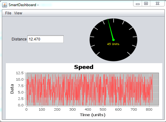
The SmartDashboard is a Java program that will display robot data in real time. The SmartDashboard helps you with these things:
Displays robot data of your choice while the program is running. It can be displayed as simple text fields or more elaborately in many other display types like graphs, dials, etc.
Displays the state of the robot program such as the currently executing commands and the status of any subsystems
Displays buttons that you can press to cause variables to be set on your robot
Allows you to choose startup options on the dashboard that can be read by the robot program
The displayed data is automatically formatted in real-time as the data is sent from the robot, but you can change the format or the display widget types and then save the new screen layouts to be used again later. And with all these options, it is still extremely simple to use. To display some data on the dashboard, simply call one of the SmartDashboard methods with the data and its name and the value will automatically appear on the dashboard screen.
Installing the SmartDashboard
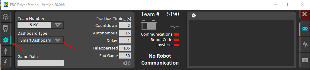
The SmartDashboard is packaged with the WPILib Installer and can be launched directly from the Driver Station by selecting the SmartDashboard button on the Setup tab.
Configuring the Team Number
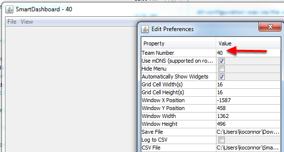
The first time you launch the SmartDashboard you should be prompted for your team number. To change the team number after this: click File > Preferences to open the Preferences dialog. Double-click the box to the right of Team Number and enter your FRC® Team Number, then click outside the box to save.
Note
SmartDashboard will take a moment to configure itself for the team number, do not be alarmed.
Setting a Custom NetworkTables Server Location
By default, SmartDashboard will look for NetworkTables instances running on a connected RoboRIO, but it’s sometimes useful to look for NetworkTables at a different IP address. To connect to SmartDashboard from a host other than the roboRIO, open SmartDashboard preferences under the File menu and in the Team Number field, enter the IP address or hostname of the NetworkTables host.
This option is incredibly useful for using SmartDashboard with WPILib simulation. Simply add localhost to the Team Number field and SmartDashboard will detect your locally-hosted robot!
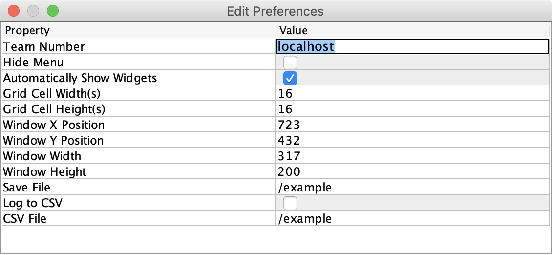
Locating the Save File
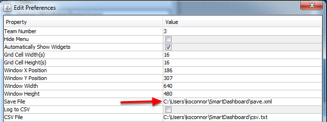
Users may wish to customize the save location of the SmartDashboard. To do this click the box next to Save File then browse to the folder where you would like to save the configuration. Files saved in the installation directories for the WPILib components will likely be overwritten on updates to the tools.
Adding a Connection Indicator
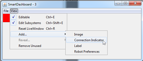
It is often helpful to see if the SmartDashboard is connected to the robot. To add a connection indicator, select View > Add > Connection Indicator. This indicator will be red when disconnected and green when connected. To move or resize this indicator, select View > Editable to toggle the SmartDashboard into editable mode, then drag the center of the indicator to move it or the edges to resize. Select the Editable item again to lock it in place.
Adding Widgets to the SmartDashboard
Widgets are automatically added to the SmartDashboard for each “key” sent by the robot code. For instructions on adding robot code to write to the SmartDashboard see Displaying Expressions from Within the Robot Program.
Displaying Expressions from a Robot Program
Note
Often debugging or monitoring the status of a robot involves writing a number of values to the console and watching them stream by. With SmartDashboard you can put values to a GUI that is automatically constructed based on your program. As values are updated, the corresponding GUI element changes value - there is no need to try to catch numbers streaming by on the screen.
Writing Values to SmartDashboard
protected void execute() {
  SmartDashboard.putBoolean("Bridge Limit", bridgeTipper.atBridge());
  SmartDashboard.putNumber("Bridge Angle", bridgeTipper.getPosition());
  SmartDashboard.putNumber("Swerve Angle", drivetrain.getSwerveAngle());
  SmartDashboard.putNumber("Left Drive Encoder", drivetrain.getLeftEncoder());
  SmartDashboard.putNumber("Right Drive Encoder", drivetrain.getRightEncoder());
  SmartDashboard.putNumber("Turret Pot", turret.getCurrentAngle());
  SmartDashboard.putNumber("Turret Pot Voltage", turret.getAverageVoltage());
  SmartDashboard.putNumber("RPM", shooter.getRPM());
}
void Command::Execute() {
  frc::SmartDashboard::PutBoolean("Bridge Limit", BridgeTipper.AtBridge());
  frc::SmartDashboard::PutNumber("Bridge Angle", BridgeTipper.GetPosition());
  frc::SmartDashboard::PutNumber("Swerve Angle", Drivetrain.GetSwerveAngle());
  frc::SmartDashboard::PutNumber("Left Drive Encoder", Drivetrain.GetLeftEncoder());
  frc::SmartDashboard::PutNumber("Right Drive Encoder", Drivetrain.GetRightEncoder());
  frc::SmartDashboard::PutNumber("Turret Pot", Turret.GetCurrentAngle());
  frc::SmartDashboard::PutNumber("Turret Pot Voltage", Turret.GetAverageVoltage());
  frc::SmartDashboard::PutNumber("RPM", Shooter.GetRPM());
}
You can write Boolean, Numeric, or String values to the SmartDashboard by simply calling the correct method for the type and including the name and the value of the data, no additional code is required. Any time in your program that you write another value with the same name, it appears in the same UI element on the screen on the driver station or development computer. As you can imagine this is a great way of debugging and getting status of your robot as it is operating.
Creating Widgets on SmartDashboard
Widgets are populated on the SmartDashboard automatically, no user intervention is required. Note that the widgets are only populated when the value is first written, you may need to enable your robot in a particular mode or trigger a particular code routine for an item to appear. To alter the appearance of the widget, see the next two sections Changing the Display Properties of a Value and Changing the Display Widget Type for a Value.
Stale Data
SmartDashboard uses NetworkTables for communicating values between the robot and the driver station laptop. NetworkTables acts as a distributed table of name and value pairs. If a name/value pair is added to either the client (laptop) or server (robot) it is replicated to the other. If a name/value pair is deleted from, say, the robot but the SmartDashboard or OutlineViewer are still running, then when the robot is restarted, the old values will still appear in the SmartDashboard and OutlineViewer because they never stopped running and continue to have those values in their tables. When the robot restarts, those old values will be replicated to the robot.
To ensure that the SmartDashboard and OutlineViewer are showing current values, it is necessary to restart the NetworkTables clients and robot at the same time. That way, old values that one is holding won’t get replicated to the others.
This usually isn’t a problem if the program isn’t constantly changing, but if the program is in development and the set of keys being added to NetworkTables is constantly changing, then it might be necessary to do the restart of everything to accurately see what is current.
Changing the display properties of a value
Each value displayed with SmartDashboard has a a set of properties that effect the way it’s displayed.
Setting the SmartDashboard display into editing mode
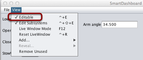
The SmartDashboard has two modes it can operate in, display mode and edit mode. In edit mode you can move around widgets on the screen and edit their properties. To put the SmartDashboard into edit mode, click the “View” menu, then select “Editable” to turn on edit mode.
Getting the properties editor of a widget
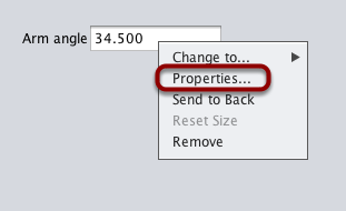
Once in edit mode, you can display and edit the properties for a widget. Right-click on the widget and select “Properties…”.
Editing the properties on a field
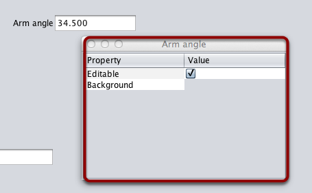
A dialog box will be shown in response to the “Properties…” menu item on the widgets right-click context menu.
Editing the widgets background color
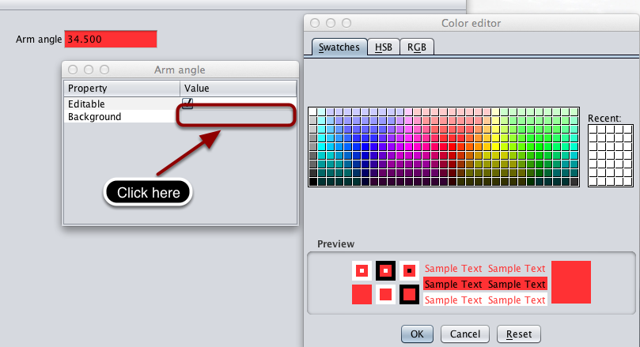
To edit a property value, say, Background color, click the background color shown (in this case grey), and choose a color from the color editor that pops up. This will be used as the widgets background color.
Edit properties of other widgets
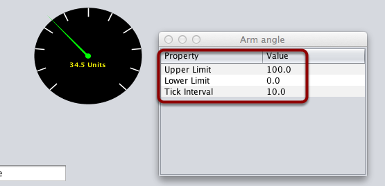
Different widget types have different sets of editable properties to change the appearance. In this example, the upper and lower limits of the dial and the tick interval are changeable parameters.
Changing the Display Widget Type for a Value
One can change the type of widget that displays values with the SmartDashboard. The allowable widgets depend on the type of the value being displayed.
Setting Edit Mode
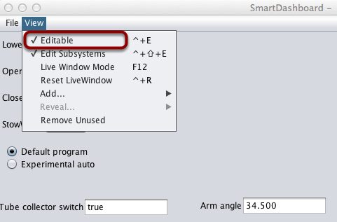
Make sure that the SmartDashboard is in edit mode. This is done by selecting Editable from the View menu.
Choosing Widget Type
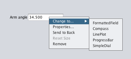
Right-click on the widget and select Change to.... Then, pick the type of widget to use for the particular value. In this case we choose LinePlot.
Showing New Widget Type
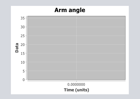
The new widget type is displayed. In this case, a Line Plot, will show the values of the Arm angle value over time. You can set the properties of the graph to make it better fit your data by right-clicking and selecting Properties.... See: Changing the display properties of a value.
Choosing an Autonomous Program
Often teams have more than one autonomous program, either for competitive reasons or for testing new software. Programs often vary by adding things like time delays, different strategies, etc. The methods to choose the strategy to run usually involves switches, joystick buttons, knobs or other hardware based inputs.
With the SmartDashboard you can simply display a widget on the screen to choose the autonomous program that you would like to run. And with command based programs, that program is encapsulated in one of several commands. This article shows how to select an autonomous program with only a few lines of code and a nice looking user interface.
Creating the SendableChooser Object
In RobotContainer, create a variable to hold a reference to a SendableChooser object. Two or more commands can be created and stored in new variables. Using the SendableChooser, one can choose between them. In this example, SimpleAuto and ComplexAuto are shown as options.
  // A simple auto routine that drives forward a specified distance, and then stops.
  private final Command m_simpleAuto =
      new DriveDistance(
          AutoConstants.kAutoDriveDistanceInches, AutoConstants.kAutoDriveSpeed, m_robotDrive);

  // A complex auto routine that drives forward, drops a hatch, and then drives backward.
  private final Command m_complexAuto = new ComplexAuto(m_robotDrive, m_hatchSubsystem);

  // A chooser for autonomous commands
  SendableChooser<Command> m_chooser = new SendableChooser<>();
  // The autonomous routines
  DriveDistance m_simpleAuto{AutoConstants::kAutoDriveDistanceInches,
                             AutoConstants::kAutoDriveSpeed, &m_drive};
  ComplexAuto m_complexAuto{&m_drive, &m_hatch};

  // The chooser for the autonomous routines
  frc::SendableChooser<frc2::Command*> m_chooser;
Setting up SendableChooser
Imagine that you have two autonomous programs to choose between and they are encapsulated in commands SimpleAuto and ComplexAuto. To choose between them:
In RobotContainer, create a SendableChooser object and add instances of the two commands to it. There can be any number of commands, and the one added as a default (setDefaultOption), becomes the one that is initially selected. Notice that each command is included in an setDefaultOption() or addOption() method call on the SendableChooser instance.
// Add commands to the autonomous command chooser
m_chooser.setDefaultOption("Simple Auto", m_simpleAuto);
m_chooser.addOption("Complex Auto", m_complexAuto);

// Put the chooser on the dashboard
SmartDashboard.putData(m_chooser);
// Add commands to the autonomous command chooser
m_chooser.SetDefaultOption("Simple Auto", &m_simpleAuto);
m_chooser.AddOption("Complex Auto", &m_complexAuto);

// Put the chooser on the dashboard
frc::SmartDashboard::PutData(&m_chooser);
Starting an Autonomous Command
In Robot.java, when the autonomous period starts, the SendableChooser object is polled to get the selected command and that command must be scheduled.
  public Command getAutonomousCommand() {
    return m_chooser.getSelected();
  }
  public void autonomousInit() {
    m_autonomousCommand = m_robotContainer.getAutonomousCommand();

    // schedule the autonomous command (example)
    if (m_autonomousCommand != null) {
      m_autonomousCommand.schedule();
    }
  }
frc2::Command* RobotContainer::GetAutonomousCommand() {
  // Runs the chosen command in autonomous
  return m_chooser.GetSelected();
}
void Robot::AutonomousInit() {
  m_autonomousCommand = m_container.GetAutonomousCommand();

  if (m_autonomousCommand != nullptr) {
    m_autonomousCommand->Schedule();
  }
}
Running the Scheduler during Autonomous
In Robot.java, this will run the scheduler every driver station update period (about every 20ms) and cause the selected autonomous command to run.
Note
Running the scheduler can occur in the autonomousPeriodic() function or robotPeriodic(), both will function similarly in autonomous mode.
40  @Override
41  public void robotPeriodic() {
42    CommandScheduler.getInstance().run();
43  }
20void Robot::RobotPeriodic() {
21  frc2::CommandScheduler::GetInstance().Run();
22}
Canceling the Autonomous Command
In Robot.java, when the teleop period begins, the autonomous command will be canceled.
78  @Override
79  public void teleopInit() {
80    // This makes sure that the autonomous stops running when
81    // teleop starts running. If you want the autonomous to
82    // continue until interrupted by another command, remove
83    // this line or comment it out.
84    if (m_autonomousCommand != null) {
85      m_autonomousCommand.cancel();
86    }
87  }
void Robot::TeleopInit() {
  // This makes sure that the autonomous stops running when
  // teleop starts running. If you want the autonomous to
  // continue until interrupted by another command, remove
  // this line or comment it out.
  if (m_autonomousCommand != nullptr) {
    m_autonomousCommand->Cancel();
    m_autonomousCommand = nullptr;
  }
}
SmartDashboard Display
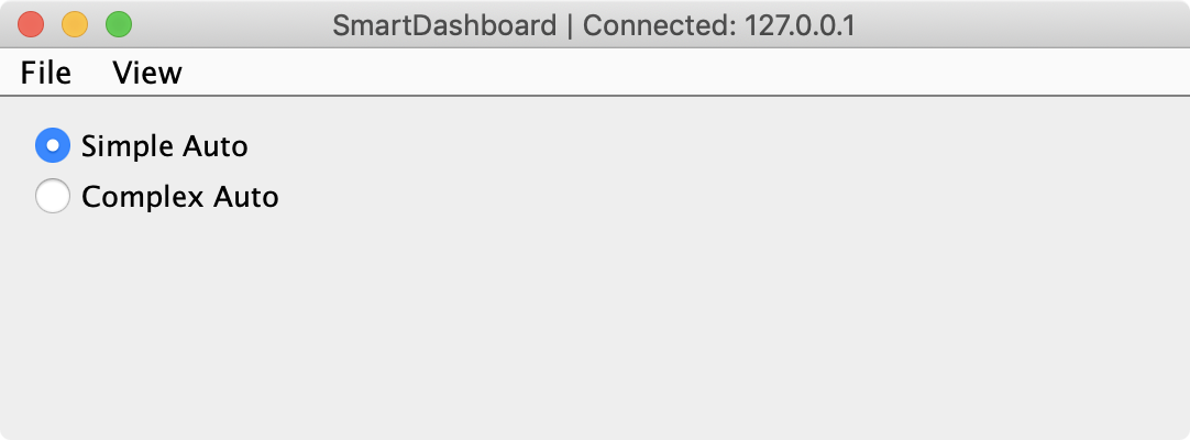
When the SmartDashboard is run, the choices from the SendableChooser are automatically displayed. You can simply pick an option before the autonomous period begins and the corresponding command will run.
Displaying the Status of Commands and Subsystems
If you are using the command-based programming features of WPILib, you will find that they are very well integrated with SmartDashboard. It can help diagnose what the robot is doing at any time and it gives you control and a view of what’s currently running.
Overview of Command and Subsystem Displays
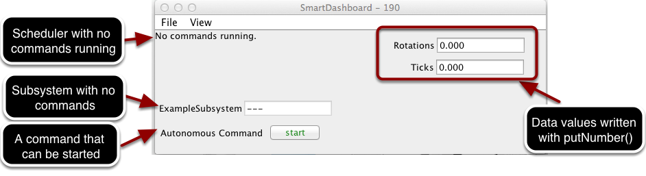
With SmartDashboard you can display the status of the commands and subsystems in your robot program in various ways. The outputs should significantly reduce the debugging time for your programs. In this picture you can see a number of displays that are possible. Displayed here are:
The Scheduler currently with
No commands running. In the next example you can see what it looks like with a few commands running showing the status of the robot.A subsystem,
ExampleSubsystemthat indicates that there are currently no commands running that are “requiring” it. When commands are running, it will indicate the name of the commands that are using the subsystem.A command written to SmartDashboard that shows a
startbutton that can be pressed to run the command. This is an excellent way of testing your commands one at a time.And a few data values written to the dashboard to help debug the code that’s running.
In the following examples, you’ll see what the screen would look like when there are commands running, and the code that produces this display.
Displaying the Scheduler Status
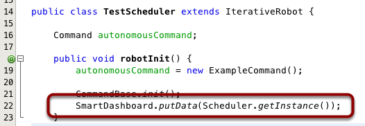
You can display the status of the Scheduler (the code that schedules your commands to run). This is easily done by adding a single line to the RobotInit method in your RobotProgram as shown here. In this example the Scheduler instance is written using the putData method to SmartDashboard. This line of code produces the display in the previous image.
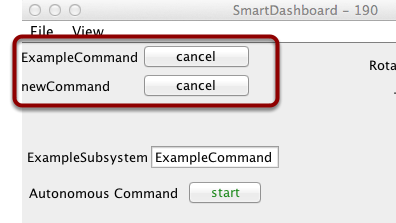
This is the scheduler status when there are two commands running, ExampleCommand and newCommand. This replaces the No commands running. message from the previous screen image. You can see commands displayed on the dashboard as the program runs and various commands are triggered.
Displaying Subsystem Status
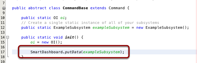
In this example we are writing the command instance, exampleSubsystem and instance of the ExampleSubsystem class to the SmartDashboard. This causes the display shown in the previous image. The text field will either contain a few dashes, --- indicating that no command is current using this subsystem, or the name of the command currently using this subsystem.
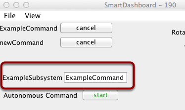
Running commands will “require” subsystems. That is the command is reserving the subsystem for its exclusive use. If you display a subsystem on SmartDashboard, it will display which command is currently using it. In this example, ExampleSubsystem is in use by ExampleCommand.
Activating Commands with a Button
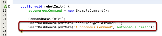
This is the code required to create a button for the command on SmartDashboard. RobotBuilder will automatically generate this code for you, but it can easily be done by hand as shown here. Pressing the button will schedule the command. While the command is running, the button label changes from start to cancel and pressing the button will cancel the command.
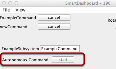
In this example you can see a button labeled Autonomous Command. Pressing this button will run the associated command and is an excellent way of testing commands one at a time without having to add throw-away test code to your robot program. Adding buttons for each command makes it simple to test the program, one command at a time.
Setting Robot Preferences
The Robot Preferences (Java, C++) class is used to store values in the flash memory on the roboRIO. The values might be for remembering preferences on the robot such as calibration settings for potentiometers, PID values, etc. that you would like to change without having to rebuild the program. The values can be viewed on the SmartDashboard and read and written by the robot program.
Reading and Writing Preferences
public class Robot extends TimedRobot {

  double armUpPosition;
  double armDownPosition;

  public void robotInit() {
    armUpPosition = Preferences.getDouble("ArmUpPosition", 1.0);
    armDownPosition = Preferences.getDouble("ArmDownPosition", 4.);
  }
}
class Robot: public TimedRobot {

  double armUpPosition;
  double armDownPosition;

  public void RobotInit() {
    armUpPosition = frc::Preferences::GetDouble("ArmUpPosition", 1.0);
    armDownPosition = frc::Preferences::GetDouble("ArmDownPosition", 4.);
  }
}
Often potentiometers are used to measure the angle of an arm or the position of some other shaft. In this case, the arm has two positions, ArmUpPosition and ArmDownPosition. Usually programmers create constants in the program that are the two pot values that correspond to the positions of the arm. When the potentiometer needs to be replaced or adjusted then the program needs to be edited and reloaded onto the robot.
Rather than having “hard-coded” values in the program the potentiometer settings can be stored in the preferences file and read by the program when it starts. In this case the values are read on program startup in the robotInit() method. These values are automatically read from the preferences file stored in the roboRIO flash memory.
Displaying Preferences in SmartDashboard
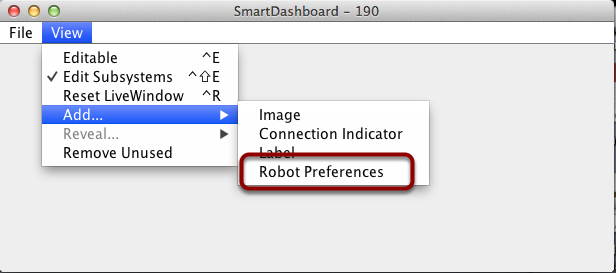
In the SmartDashboard, the Preferences display can be added to the display revealing the contents of the preferences file stored in the roboRIO flash memory.
Viewing and Editing Preferences
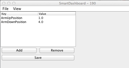
The values are shown here with the default values from the code. This was read from the robot through the NetworkTables interface built into SmartDashboard. If the values need to be adjusted they can be edited here and saved. The next time the robot program starts up the new values will be loaded in the robotInit() method. Each subsequent time the robot starts, the new values will be retrieved without having to edit and recompile/reload the robot program.
Verifying SmartDashboard is working
Connection Indicator
SmartDashboard will automatically include the connection status and IP address of the NetworkTables source in the title of the window.
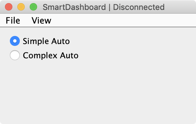
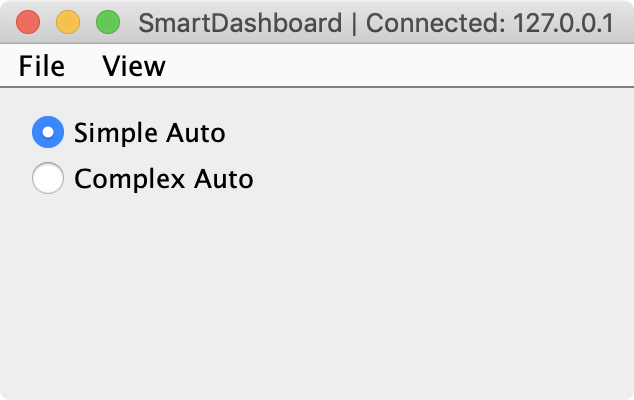
Connection Indicator Widget
SmartDashboard includes a connection indicator widget which will turn red or green depending on the connection to NetworkTables, usually provided by the roboRIO. For instructions to add this widget, look at Adding a Connection Indicator in the SmartDashboard Intro.
Robot Program Example
public class Robot extends TimedRobot {
  double counter = 0.0;

  public void teleopPeriodic() {
    SmartDashboard.putNumber("Counter", counter++);
  }
}
#include "Robot.h"
float counter = 0.0;

void Robot::TeleopPeriodic() {
    frc::SmartDashboard::PutNumber("Counter", counter++);
}
This is a minimal robot program that writes a value to the SmartDashboard. It simply increments a counter 50 times per second to verify that the connection is working. However, to minimize bandwidth usage, NetworkTables by default will throttle the updates to 10 times per second.
SmartDashboard Output for the Sample Program
The SmartDashboard display should look like this after about 6 seconds of the robot being enabled in Teleop mode. If it doesn’t, then you need to check that the connection is correctly set up.
Verifying the IP address in SmartDashboard
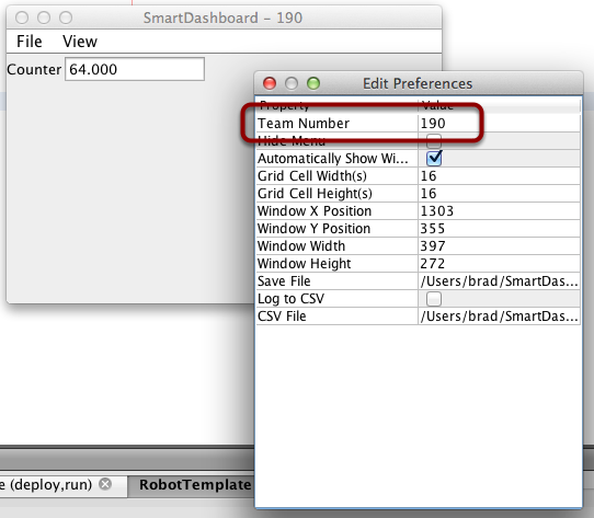
If the display of the value is not appearing, verify that the team number is correctly set as shown in this picture. The preferences dialog can be viewed by selecting File, then Preferences.
Verifying Program using OutlineViewer
You can verify that the robot program is generating SmartDashboard values by using the OutlineViewer program. This is a Java program, OutlineViewer.jar, that is located in ~/wpilib/YYYY/tools (where YYYY is the year and ~ is C:\Users\Public on Windows).
OutlineViewer is downloaded as part of the WPILib Offline Installer. For more information, see the Windows/macOS/Linux installation guides. In Visual Studio Code, press Ctrl+Shift+P and type “WPILib” or click the WPILib logo in the top right to launch the WPILib Command Palette. Select Start Tool, and then select OutlineViewer.
In the “Server Location” box, enter your team number with no leading zeroes. Then, click Start.
Look at the second row in the table, the value SmartDashboard/Counter is the variable written to the SmartDashboard via NetworkTables. As the program runs you should see the value increasing (41.0 in this case). If you don’t see this variable in the OutlineViewer, look for something wrong with the robot program or the network configuration.
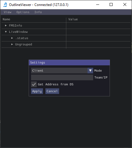
SmartDashboard Namespace
SmartDashboard uses NetworkTables to send data between the robot and the Dashboard (Driver Station) computer. NetworkTables sends data as name, value pairs, like a distributed hashtable between the robot and the computer. When a value is changed in one place, its value is automatically updated in the other place. This mechanism and a standard set of name (keys) is how data is displayed on the SmartDashboard.
There is a hierarchical structure in the name space creating a set of tables and subtables. SmartDashboard data is in the SmartDashboard subtable and LiveWindow data is in the LiveWindow subtable as shown below.
For informational purposes, the names and values can be displayed using the OutlineViewer application that is installed in the same location as the SmartDashboard. It will display all the NetworkTables keys and values as they are updated.
SmartDashboard Data Values
SmartDashboard values are created with key names that begin with SmartDashboard/. The above values viewed with OutlineViewer correspond to data put to the SmartDashboard with the following statements:
chooser = new SendableChooser();
chooser.setDefaultOption("defaultAuto", new AutonomousCommand());
chooser.addOption("secondAuto", new AutonomousCommand());
chooser.addOption("thirdAuto", new AutonomousCommand());
SmartDashboard.putData("Chooser", chooser);
SmartDashboard.putNumber("Arm position in degrees", 52.0);
SmartDashboard.putString("Program Version", "V1.2");
The Arm position is created with the putNumber() call. The AutonomousCommand is written with a putData("Autonomous Command", command) that is not shown in the above code fragment. The chooser is created as a SendableChooser object and the string value, Program Version is created with the putString() call.
View of SmartDashboard
The code from the previous step generates the table values as shown and the SmartDashboard display as shown here. The numbers correspond to the NetworkTables variables shown in the previous step.
LiveWindow Data Values
LiveWindow data is automatically grouped by subsystem. The data is viewable in the SmartDashboard when the robot is in Test mode (set on the Driver Station). If you are not writing a command based program, you can still cause sensors and actuators to be grouped for easy viewing by specifying the subsystem name. In the above display you can see the key names and the resultant output in Test mode on the SmartDashboard. All the strings start with /LiveWindow then the Subsystem name, then a group of values that are used to display each element. The code that generates this LiveWindow display is shown below:
drivetrainLeft = new PWMVictorSPX(1);
drivetrainLeft.setName("Drive train", "Left");

drivetrainRight = new PWMVictorSPX(1);
drivetrainRight.setName("Drive train", "Right";

drivetrainRobotDrive = new DifferentialDrive(drivetrainLeft, drivetrainRight);
drivetrainRobotDrive.setSafetyEnabled(false);
drivetrainRobotDrive.setExpiration(0.1);

drivetrainUltrasonic = new AnalogInput(3);
drivetrainUltrasonic.setName("Drive train", "Ultrasonic");

elevatorMotor = new PWMVictorSPX(6);
elevatorMotor.setName("Elevator", "Motor");

elevatorPot = new AnalogInput(4);
elevatorPot.setName("Elevator", "Pot");

wristPot = new AnalogInput(2);
wristPot.setName("Wrist", "Pot");

wristMotor = new PWMVictorSPX(3);
wristMotor.setName("Wrist", "Motor");

clawMotor = new PWMVictorSPX(5);
clawMotor.setName("Claw", "Motor");
Values that correspond to actuators are not only displayed, but can be set using sliders created in the SmartDashboard in Test mode.
SmartDashboard: Test Mode and Live Window
Displaying LiveWindow Values
Note
LiveWindow will automatically add your sensors for you. There is no need to do it manually.
LiveWindow values may also be displayed by writing the code yourself and adding it to your robot program. LiveWindow will display values grouped in subsystems. This is a convenient method of displaying whether they are actual command based program subsystems or just a grouping that you decide to use in your program.
Adding the Necessary Code to your Program
For each sensor or actuator that is created, set the subsystem name and display name by calling setName (SetName in C++). When the SmartDashboard is put into LiveWindow mode, it will display the sensors and actuators.
Ultrasonic ultrasonic = new Ultrasonic(1, 2);
ultrasonic.setName("Arm", "Ultrasonic");

Jaguar elbow = new Jaguar(1);
elbow.setName("Arm", "Elbow");

Victor wrist = new Victor(2);
wrist.setName("Arm", "Wrist");
frc::Ultrasonic ultrasonic{1, 2};
ultrasonic.SetName("Arm", "Ultrasonic");

frc::Jaguar elbow{1};
elbow.SetName("Arm", "Elbow");

frc::Victor wrist{2};
wrist.SetName("Arm", "Wrist");
Viewing the Display in SmartDashboard
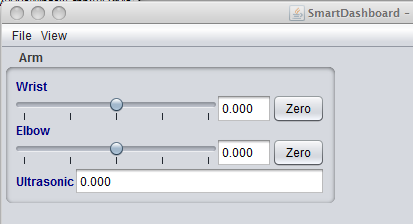
The sensors and actuators added to the LiveWindow will be displayed grouped by subsystem. The subsystem name is just an arbitrary grouping the helping to organize the display of the sensors. Actuators can be operated by operating the slider for the two motor controllers.
Enabling Test mode (LiveWindow)
You may add code to your program to display values for your sensors and actuators while the robot is in Test mode. This can be selected from the Driver Station whenever the robot is not on the field. The code to display these values is automatically generated by RobotBuilder and is described in the next article. Test mode is designed to verify the correct operation of the sensors and actuators on a robot. In addition it can be used for obtaining setpoints from sensors such as potentiometers and for tuning PID loops in your code.
Setting Test mode with the Driver Station
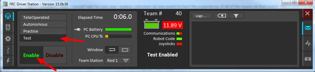
Enable Test Mode in the Driver Station by clicking on the “Test” button and setting “Enable” on the robot. When doing this, the SmartDashboard display will switch to test mode (LiveWindow) and will display the status of any actuators and sensors used by your program.
Explicitly vs. implicit test mode display
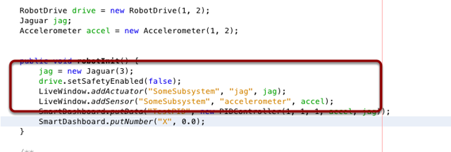
All sensors and actuators will automatically be displayed on the SmartDashboard in test mode and will be named using the object type (such as Jaguar, Analog, Victor, etc.) with the module number and channel number with which the object was created. In addition, the program can explicitly add sensors and actuators to the test mode display, in which case programmer-defined subsystem and object names can be specified making the program clearer. This example illustrates explicitly defining those sensors and actuators in the highlighted code.
Understanding what is displayed in Test mode
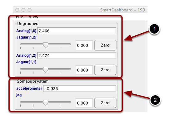
This is the output in the SmartDashboard display when the robot is placed into test mode. In the display shown above the objects listed as Ungrouped were implicitly created by WPILib when the corresponding objects were created. These objects are contained in a subsystem group called “Ungrouped” (1) and are named with the device type (Analog, Jaguar in this case), and the module and channel numbers. The objects shown in the “SomeSubsystem” (2) group are explicitly created by the programmer from the code example in the previous section. These are named in the calls to LiveWindow.addActuator() and LiveWindow.AddSensor(). Explicitly created sensors and actuators will be grouped by the specified subsystem.
PID Tuning with SmartDashboard
The PID (Proportional, Integral, Differential) is an algorithm for determining the motor speed based on sensor feedback to reach a setpoint as quickly as possible. For example, a robot with an elevator that moves to a predetermined position should move there as fast as possible then stop without excessive overshoot leading to oscillation. Getting the PID controller to behave this way is called “tuning”. The idea is to compute an error value that is the difference between the current value of the mechanism feedback element and the desired (setpoint) value. In the case of the arm, there might be a potentiometer connected to an analog channel that provides a voltage that is proportional to the position of the arm. The desired value is the voltage that is predetermined for the position the arm should move to, and the current value is the voltage for the actual position of the arm.
Finding the setpoint values with LiveWindow
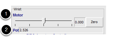
Create a PID Subsystem for each mechanism with feedback. The PID Subsystems contain the actuator (motor) and the feedback sensor (potentiometer in this case). You can use Test mode to display the subsystem sensors and actuators. Using the slider manually adjust the actuator to each desired position. Note the sensor values (2) for each of the desired positions. These will become the setpoints for the PID controller.
Viewing the PIDController in LiveWindow
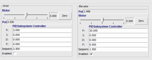
In Test mode, the PID Subsystems display their P, I, and D parameters that are set in the code. The P, I, and D values are the weights applied to the computed error (P), sum of errors over time (I), and the rate of change of errors (D). Each of those terms is multiplied by the weights and added together to form the motor value. Choosing the optimal P, I, and D values can be difficult and requires some amount of experimentation. The Test mode on the robot allows the values to be modified, and the mechanism response observed.
Important
The enable option does not affect the PIDController introduced in 2020, as the controller is updated every robot loop. See the example here on how to retain this fuctionality.
Tuning the PIDController
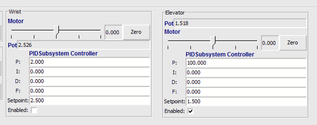
Tuning the PID controller can be difficult and there are many articles that describe techniques that can be used. It is best to start with the P value first. To try different values fill in a low number for P, enter a setpoint determined earlier in this document, and note how fast the mechanism responds. If it responds too slowly, perhaps never reaching the setpoint, increase P. If it responds too quickly, perhaps oscillating, reduce the P value. Repeat this process until you get a response that is as fast as possible without oscillation. It’s possible that having a P term is all that’s needed to achieve adequate control of your mechanism. Further information is located in the Tuning a PID Controller document.
Once you have determined P, I, and D values they can be inserted into the program. You’ll find them either in the properties for the PIDSubsystem in RobotBuilder or in the constructor for the PID Subsystem in your code.
The F (feedforward) term is used for controlling velocity with a PID controller.
More information can be found at PID Control in WPILib.
Glass
Glass is a new dashboard and robot data visualization tool. Its GUI is extremely similar to that of the Simulation GUI. In its current state, it is meant to be used as a programmer’s tool rather than a proper dashboard in a competition environment.
Note
Glass will not be available within the list of dashboards in the NI Driver Station.
Introduction to Glass
Glass is a new dashboard and robot data visualization tool. It supports many of the same widgets that the Simulation GUI supports, including robot pose visualization and advanced plotting. In its current state, it is meant to be used as a programmer’s tool for debugging and not as a dashboard for competition use.
Opening Glass
Glass can be launched by selecting the ellipsis menu (…) in VS Code, clicking on Start Tool and then choosing Glass.
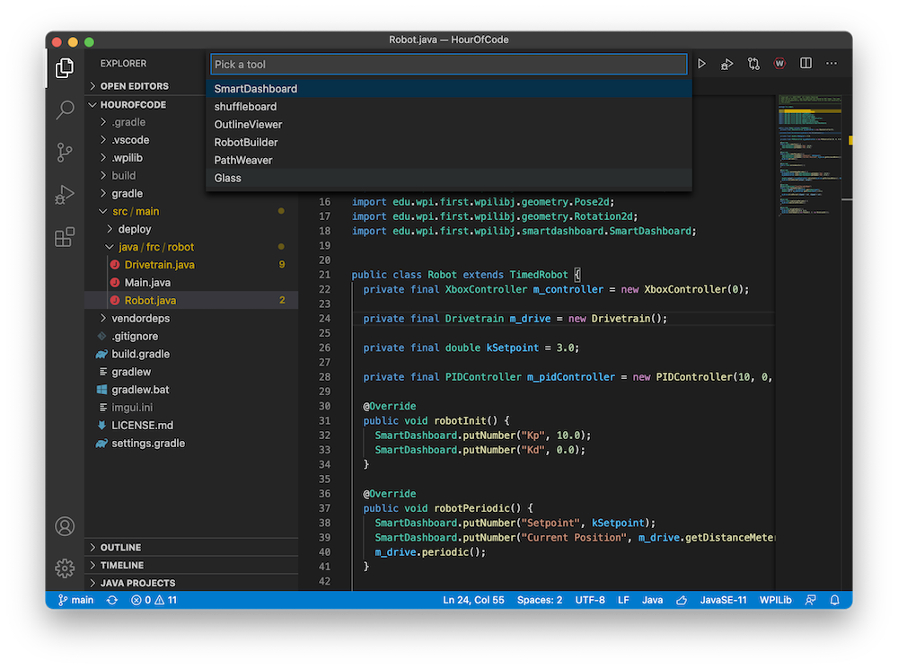
Note
You can also launch Glass directly by navigating to ~/wpilib/YYYY/tools and running Glass.py (Linux and macOS) or by using the shortcut inside the WPILib Tools desktop folder (Windows).
Changing View Settings
The View menu item contains Zoom and Style settings that can be customized. The Zoom option dictates the size of the text in the application whereas the Style option allows you to select between the Classic, Light, and Dark modes.
An example of the Dark style setting is below:
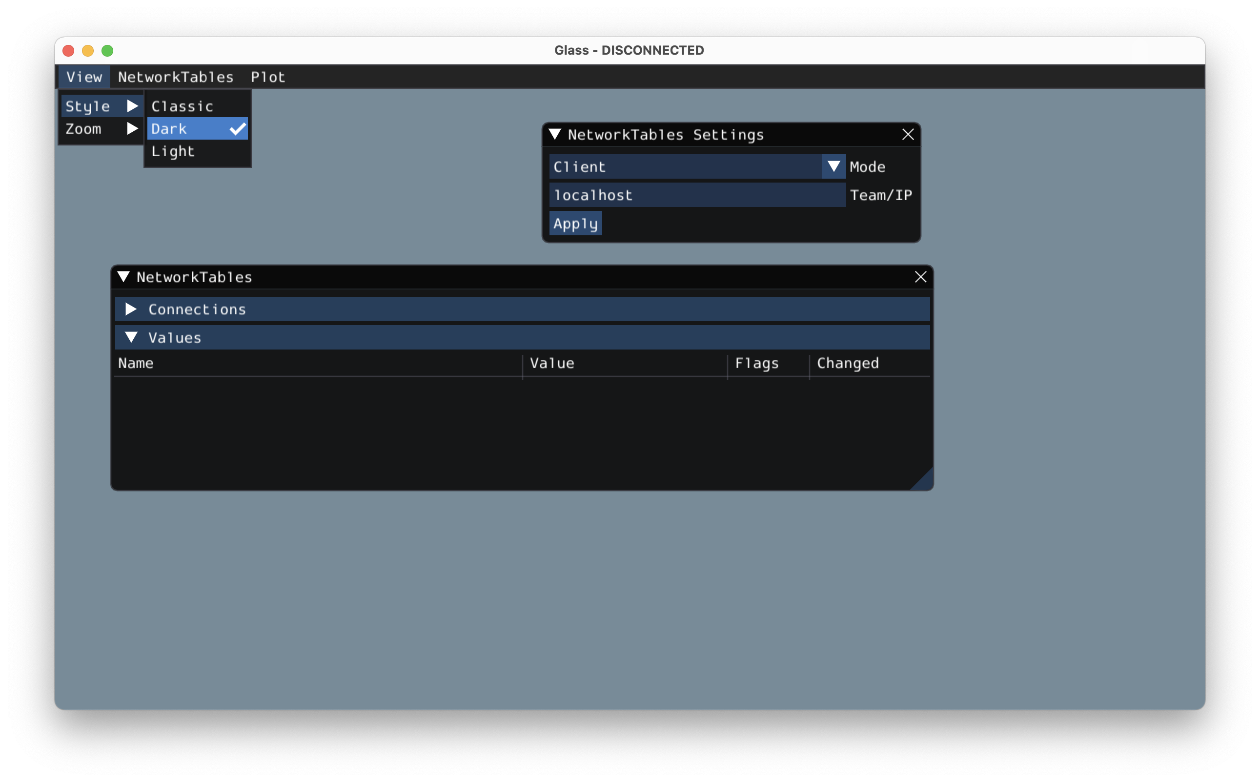
Clearing Application Data
Application data for Glass, including widget sizes and positions as well as other custom information for widgets is stored in a glass.ini file. The location of this file varies based on your operating system:
On Windows, the configuration file is located in
%APPDATA%.On macOS, the configuration file is located in
~/Library/Preferences.On Linux, the configuration file is located in
$XDG_CONFIG_HOMEor~/.configif the former does not exist.
The glass.ini configuration file can simply be deleted to restore Glass to a “clean slate”.
Establishing NetworkTables Connections
Glass uses the NetworkTables protocol to establish a connection with your robot program. It is also used to transmit and receive data to and from the robot.
Connecting to a Robot
When Glass is first launched, you will see two widgets – NetworkTables Settings and NetworkTables. To connect to a robot, select Client under Mode in the NetworkTables Settings widget, enter your team number and click on Apply.
You can also connect to a robot that is running in simulation on your computer (including Romi robots) by typing in localhost into the Team/IP box.
Important
The NetworkTables connection status is always visible on the title bar of the Glass application.
Viewing NetworkTables Entries
The NetworkTables widget can be used to view all entries that are being sent over NetworkTables. These entries are hierarchically arranged by main table, sub-table, and so on.
Furthermore, you can view all connected NetworkTables clients under the Connections pane of the widget.
Glass Widgets
Specialized widgets are available for certain types that exist in robot code. These include objects that are manually sent over NetworkTables such as SendableChooser instances, or hardware that is automatically sent over LiveWindow.
Note
Widget support in Glass is still in its infancy – therefore, there are only a handful of widgets available. This list will grow as development work continues.
Note
A widget can be renamed by right-clicking on its header and specifying a new name.
Hardware Widgets
Widgets for specific hardware (such as motor controllers) are usually available via LiveWindow. These can be accessed by selecting the NetworkTables menu option, clicking on LiveWindow and choosing the desired widget.
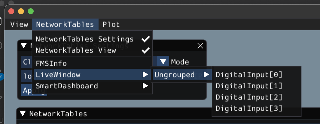
The list of hardware (sent over LiveWindow automatically) that has widgets is below:
DigitalInput
DigitalOutput
SpeedController
Gyro
Here is an example of the widget for gyroscopes:
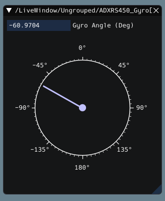
Sendable Chooser Widget
The Sendable Chooser widget represents a SendableChooser instance from robot code. It is often used to select autonomous modes. Like other dashboards, your SendableChooser instance simply needs to be sent using a NetworkTables API. The simplest is to use something like SmartDashboard:
SmartDashboard.putData("Auto Selector", m_selector);
frc::SmartDashboard::PutData("Auto Selector", &m_selector);
Note
For more information on creating a SendableChooser, please see this document.
The Sendable Chooser widget will appear in the NetworkTables menu and underneath the main table name that the instance was sent over. From the example above, the main table name would be SmartDashboard.
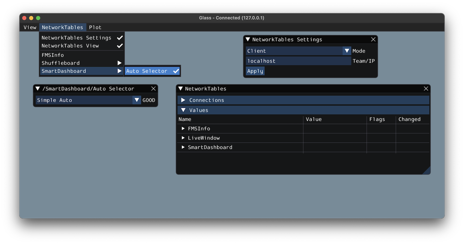
PID Controller Widget
The PID Controller widget allows you to quickly tune PID values for a certain controller. A PIDController instance must be sent using a NetworkTables API. The simplest is to use something like SmartDashboard:
SmartDashboard.putData("Elevator PID Controller", m_elevatorPIDController);
frc::SmartDashboard::PutData("Elevator PID Controller", &m_elevatorPIDController);
This allows you to quickly tune P, I, and D values for various setpoints.
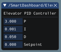
FMSInfo Widget
The FMSInfo widget is created by default when Glass connects to a robot. This widget displays basic information about the robot’s enabled state, whether a Driver Station is connected, whether an FMS is connected, the game-specific data, etc. It can be viewed by selecting the NetworkTables menu item and clicking on FMSInfo.
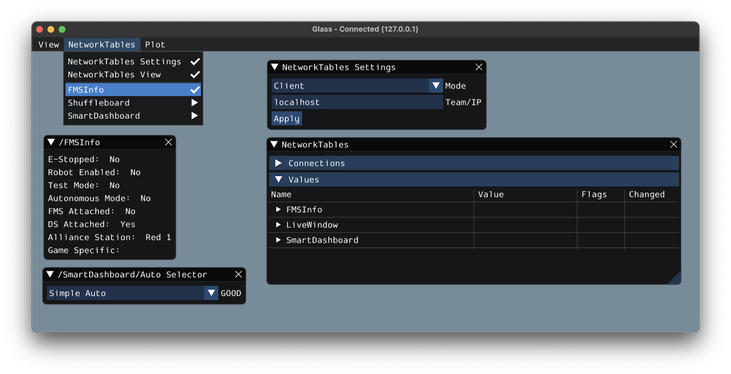
Widgets for the Command-Based Framework
Glass also has several widgets that are specific to the command-based framework. These include widgets to schedule commands, view actively running commands on a specific subsystem, or view the state of the command scheduler.
Command Selector Widget
The Command Selector widget allows you to start and cancel a specific instance of a command (sent over NetworkTables) from Glass. For example, you can create an instance of MyCommand and send it to SmartDashboard:
MyCommand command = new MyCommand(...);
SmartDashboard.putData("My Command", command);
#include <frc/smartdashboard/SmartDashboard.h>

...

MyCommand command{...};
frc::SmartDashboard::PutData("My Command", &command);
Note
The MyCommand instance can also be sent using a lower-level NetworkTables API or using the Shuffleboard API. In this case, the SmartDashboard API was used, meaning that the Command Selector widget will appear under the SmartDashboard table name.
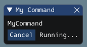
The widget has two states. When the command is not running, a Run button will appear – clicking it will schedule the command. When the command is running, a Cancel button, accompanied by Running… text, will appear (as shown above). This will cancel the command.
Subsystem Widget
The Subsystem widget can be used to see the default command and the currently scheduled command on a specific subsystem. If you are using the SubsystemBase base class, your subsystem will be automatically sent to NetworkTables over LiveWindow. To view this widget, look under the LiveWindow main table name in the NetworkTables menu.
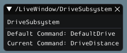
Command Scheduler Widget
The Command Scheduler widget allows you to see all currently scheduled commands. In addition, any of these commands can be canceled from the GUI.
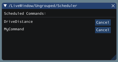
The CommandScheduler instance is automatically sent to NetworkTables over LiveWindow. To view this widget, look under the LiveWindow main table name in the NetworkTables menu.
The Field2d Widget
Glass supports displaying your robot’s position on the field using the Field2d widget. An instance of the Field2d class should be created, sent over NetworkTables, and updated periodically with the latest robot pose in your robot code.
Sending Robot Pose from User Code
To send your robot’s position (usually obtained by odometry or a pose estimator), a Field2d instance must be created in robot code and sent over NetworkTables. The instance must then be updated periodically with the latest robot pose.
private final Field2d m_field = new Field2d();

public Drivetrain() {
  ...
  SmartDashboard.putData("Field", m_field);
}

...

public void periodic() {
  ...
  m_field.setRobotPose(m_odometry.getPoseMeters());
}
#include <frc/smartdashboard/Field2d.h>
#include <frc/smartdashboard/SmartDashboard.h>

frc::Field2d m_field;

Drivetrain() {
  ...
  frc::SmartDashboard::PutData("Field", &m_field);
}

...

void Periodic() {
  ...
  m_field.SetRobotPose(m_odometry.GetPose());
}
Note
The Field2d instance can also be sent using a lower-level NetworkTables API or using the Shuffleboard API. In this case, the SmartDashboard API was used, meaning that the Field2d widget will appear under the SmartDashboard table name.
Sending Trajectories to Field2d
Visualizing your trajectory is a great debugging step for verifying that your trajectories are created as intended. Trajectories can be easily visualized in Field2d using the setTrajectory()/SetTrajectory() functions.
44  @Override
45  public void robotInit() {
46    // Create the trajectory to follow in autonomous. It is best to initialize
47    // trajectories here to avoid wasting time in autonomous.
48    m_trajectory =
49        TrajectoryGenerator.generateTrajectory(
50            new Pose2d(0, 0, Rotation2d.fromDegrees(0)),
51            List.of(new Translation2d(1, 1), new Translation2d(2, -1)),
52            new Pose2d(3, 0, Rotation2d.fromDegrees(0)),
53            new TrajectoryConfig(Units.feetToMeters(3.0), Units.feetToMeters(3.0)));
54
55    // Create and push Field2d to SmartDashboard.
56    m_field = new Field2d();
57    SmartDashboard.putData(m_field);
58
59    // Push the trajectory to Field2d.
60    m_field.getObject("traj").setTrajectory(m_trajectory);
61  }
18  void AutonomousInit() override {
19    // Start the timer.
20    m_timer.Start();
21
22    // Send Field2d to SmartDashboard.
23    frc::SmartDashboard::PutData(&m_field);
24
25    // Reset the drivetrain's odometry to the starting pose of the trajectory.
26    m_drive.ResetOdometry(m_trajectory.InitialPose());
27
28    // Send our generated trajectory to Field2d.
29    m_field.GetObject("traj")->SetTrajectory(m_trajectory);
30  }
Viewing Trajectories with Glass
The sent trajectory can be viewed with Glass through the dropdown NetworkTables -> SmartDashboard -> Field2d.
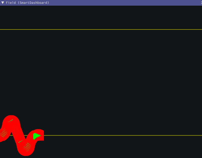
Note
The above example which uses the RamseteController (Java)/RamseteController (C++) will not show the sent trajectory until autonomous is enabled at least once.
Viewing the Robot Pose in Glass
After sending the Field2d instance over NetworkTables, the Field2d widget can be added to Glass by selecting NetworkTables in the menu bar, choosing the table name that the instance was sent over, and then clicking on the Field button.
Once the widget appears, you can resize and place it on the Glass workspace as you desire. Right-clicking the top of the widget will allow you to customize the name of the widget, select a custom field image, select a custom robot image, and choose the dimensions of the field and robot.
When selecting Choose image… you can choose to either select an image file or a PathWeaver JSON file as long as the image file is in the same directory. Choosing the JSON file will automatically import the correct location of the field in the image and the correct size of the field.
Note
You can retrieve the latest field image and JSON files from here. This is the same image and JSON that are used when generating paths using PathWeaver.
Modifying Pose Style
Poses can be customized in a plethora of ways by right clicking on the Field2d menu bar. Examples of customization are: line width, line weight, style, arrow width, arrow weight, color, etc.
One usage of customizing the pose style is converting the previously shown traj pose object to a line, rather than a list of poses. Click on the Style dropdown box and select Line. You should notice an immediate change in how the trajectory looks.
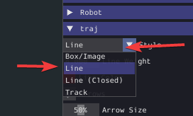
Now, uncheck the Arrows checkbox. This will cause cause our trajectory to look like a nice and fluid line!
The Mechanism2d Widget
Glass supports displaying stick-figure representations of your robot’s mechanisms using the Mechanism2d widget. It supports combinations of ligaments that can rotate and / or extend or retract, such as arms and elevators and they can be combined for more complicated mechanisms. An instance of the Mechanism2d class should be created and populated, sent over NetworkTables, and updated periodically with the latest mechanism states in your robot code. It can also be used with the Physics Simulation to visualize and program your robot’s mechanisms before the robot is built.
Creating and Configuring the Mechanism2d Instance
The Mechanism2d object is the “canvas” where the mechanism is drawn. The root node is where the mechanism is anchored to Mechanism2d. For a single jointed arm this would the pivot point. For an elevator, this would be where it’s attached to the robot’s base. To get a root node (represented by a MechanismRoot2d object), call getRoot(name, x, y) on the container Mechanism2d object. The name is used to name the root within NetworkTables, and should be unique, but otherwise isn’t important. The x / y coordinate system follows the same orientation as Field2d - (0,0) is bottom left.
In the examples below, an elevator is drawn, with a rotational wrist on top of the elevator. The full Mechanism2d example is available in Java / C++
43    // the main mechanism object
44    Mechanism2d mech = new Mechanism2d(3, 3);
45    // the mechanism root node
46    MechanismRoot2d root = mech.getRoot("climber", 2, 0);
59  // the main mechanism object
60  frc::Mechanism2d m_mech{3, 3};
61  // the mechanism root node
62  frc::MechanismRoot2d* m_root = m_mech.GetRoot("climber", 2, 0);
Each MechanismLigament2d object represents a stage of the mechanism. It has a three required parameters, a name, an initial length to draw (relative to the size of the Mechanism2d object), and an initial angle to draw the ligament in degrees. Ligament angles are relative to the parent ligament, and follow math notation - the same as Rotation2d (counterclockwise-positive). A ligament based on the root with an angle of zero will point right. Two optional parameters let you change the width (also relative to the size of the Mechanism2d object) and the color. Call append()/Append() on a root node or ligament node to add another node to the figure. In Java, pass a constructed MechanismLigament2d object to add it. In C++, pass the construction parameters in order to construct and add a ligament.
48    // MechanismLigament2d objects represent each "section"/"stage" of the mechanism, and are based
49    // off the root node or another ligament object
50    m_elevator = root.append(new MechanismLigament2d("elevator", kElevatorMinimumLength, 90));
51    m_wrist =
52        m_elevator.append(
53            new MechanismLigament2d("wrist", 0.5, 90, 6, new Color8Bit(Color.kPurple)));
63  // MechanismLigament2d objects represent each "section"/"stage" of the
64  // mechanism, and are based off the root node or another ligament object
65  frc::MechanismLigament2d* m_elevator =
66      m_root->Append<frc::MechanismLigament2d>("elevator", 1, 90_deg);
67  frc::MechanismLigament2d* m_wrist =
68      m_elevator->Append<frc::MechanismLigament2d>(
69          "wrist", 0.5, 90_deg, 6, frc::Color8Bit{frc::Color::kPurple});
Then, publish the Mechanism2d object to NetworkTables:
55    // post the mechanism to the dashboard
56    SmartDashboard.putData("Mech2d", mech);
36    // publish to dashboard
37    frc::SmartDashboard::PutData("Mech2d", &m_mech);
Note
The Mechanism2d instance can also be sent using a lower-level NetworkTables API or using the Shuffleboard API. In this case, the SmartDashboard API was used, meaning that the Mechanism2d widget will appear under the SmartDashboard table name.
To manipulate a ligament angle or length, call setLength() or setAngle() on the MechanismLigament2d object. When manipulating ligament length based off of sensor measurements, make sure to add the minimum length to prevent 0-length (and therefore invisible) ligaments.
59  @Override
60  public void robotPeriodic() {
61    // update the dashboard mechanism's state
62    m_elevator.setLength(kElevatorMinimumLength + m_elevatorEncoder.getDistance());
63    m_wrist.setAngle(m_wristPot.get());
64  }
40  void RobotPeriodic() override {
41    // update the dashboard mechanism's state
42    m_elevator->SetLength(kElevatorMinimumLength +
43                          m_elevatorEncoder.GetDistance());
44    m_wrist->SetAngle(units::degree_t(m_wristPotentiometer.Get()));
45  }
Viewing the Mechanism2d in Glass
After sending the Mechanism2d instance over NetworkTables, the Mechanism2d widget can be added to Glass by selecting NetworkTables in the menu bar, choosing the table name that the instance was sent over, and then clicking on the Field button.
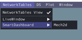
Once the widget appears as shown below, you can resize and place it on the Glass workspace as you desire. Right-clicking the top of the widget will allow you to customize the name of the widget. As the wrist potentiometer and elevator encoder changes, the mechanism will update in the widget.
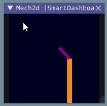
Next Steps
As mentioned above, the Mechanism2d visualization can be combined with Physics Simulation to help you program mechanisms before your robot is built. The ArmSimulation (Java / C++) and ElevatorSimulation (Java / C++) examples combine physics simulation and Mechanism2d visualization so that you can practice programing a single jointed arm and elevator without a robot.
Plots
Glass excels at high-performance, comprehensive plotting of data from NetworkTables. Some features include resizable plots, plots with multiple y axes and the ability to pause, examine, and resume plots.
Creating a Plot
A new plot widget can be created by selecting the Plot button on the main menu bar and then clicking on New Plot Window. Several individual plots can be added to each plot window. To add a plot within a plot window, click the Add plot button inside the widget. Then you can drag various sources from the NetworkTables widget into the plot:
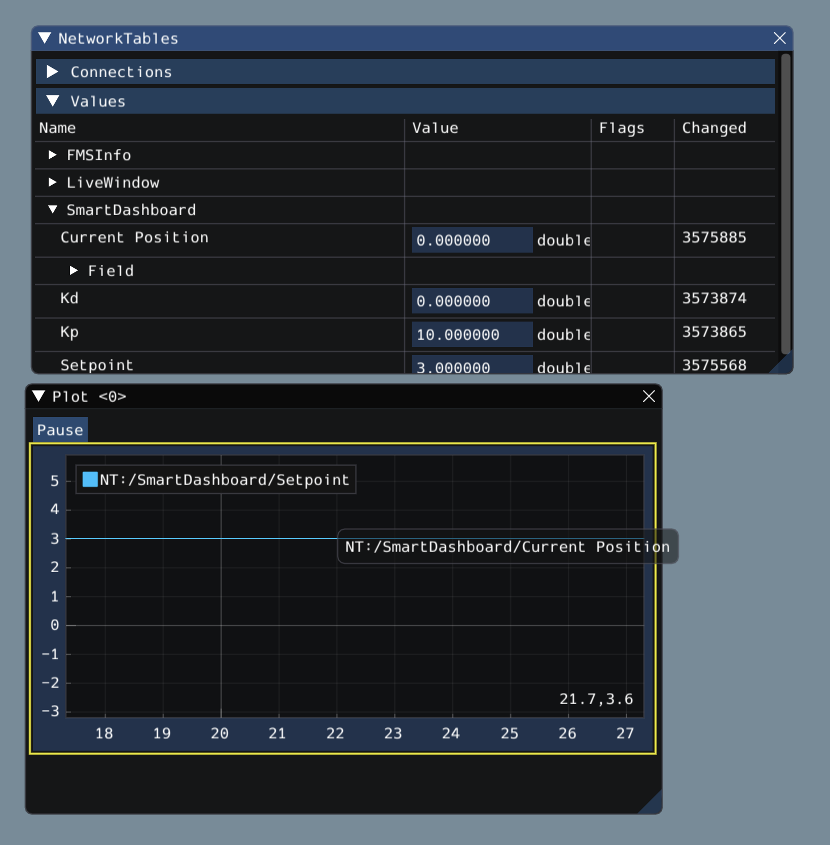
Manipulating Plots
You can click and drag on the plot to move around and scroll on top of the plot to zoom the y axes in and out. Double clicking on the graph will autoscale it so that the zoom and axis limits fit all of the data it is plotting. Furthermore, right-clicking on the plot will present you with a plethora of options, including whether you want to display secondary and tertiary y axes, if you wish to lock certain axes, etc.
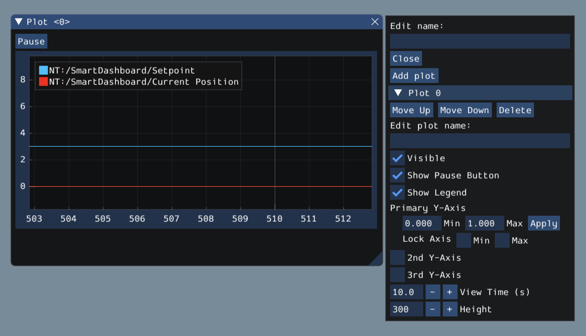
If you choose to make secondary and tertiary y axes available, you can drag data sources onto those axes to make their lines correspond with your desired axis:
Then, you can lock certain axes so that their range always remains constant, regardless of panning. In this example, the secondary axis range (with the /SmartDashboard/Kp entry) was locked between 9 and 12.
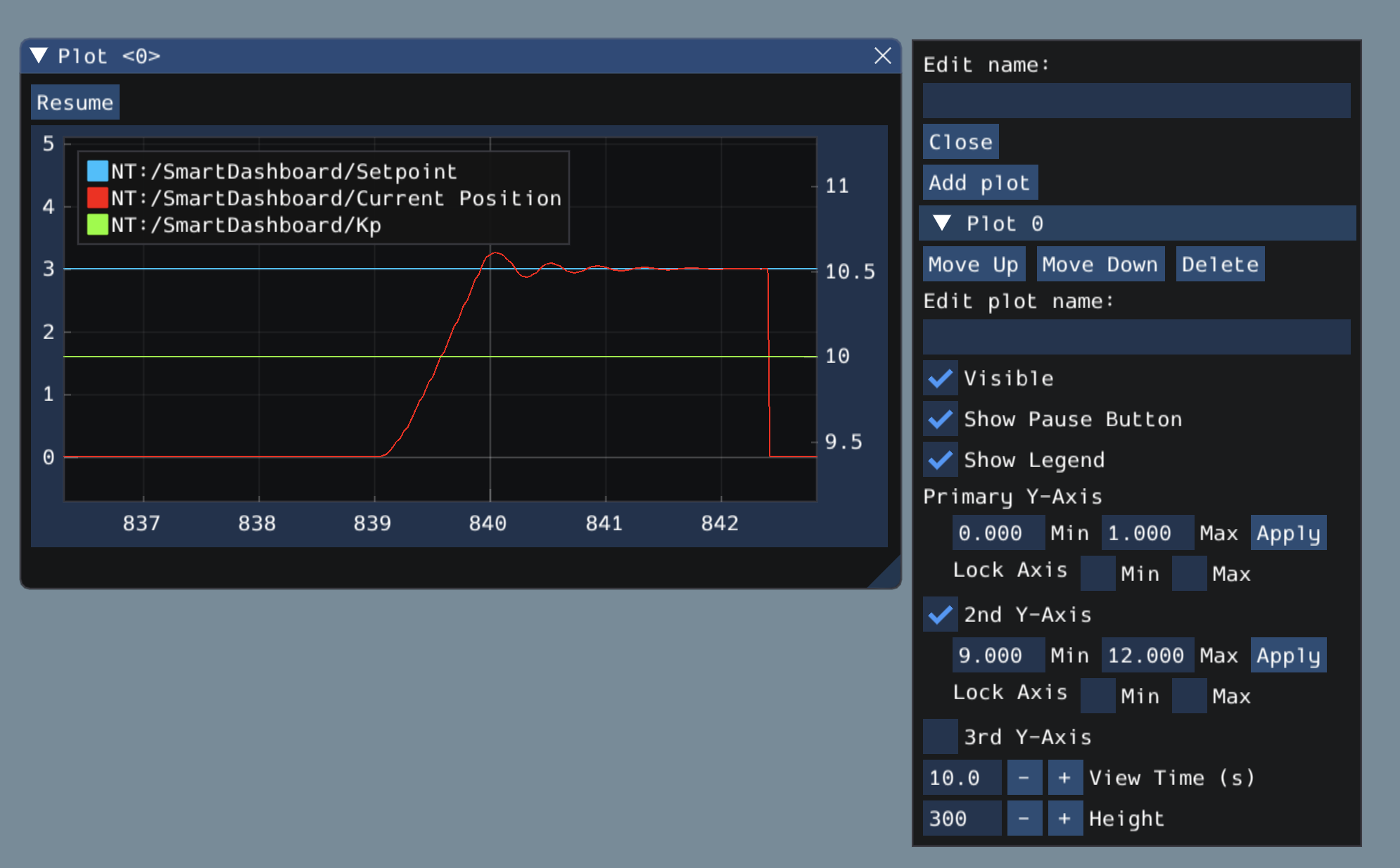
LabVIEW Dashboard
FRC LabVIEW Dashboard
The Dashboard application installed and launched by the FRC® Driver Station is a LabVIEW program designed to provide teams with basic feedback from their robot, with the ability to expand and customize the information to suit their needs. This Dashboard application uses NetworkTables and contains a variety of tools that teams may find useful.
LabVIEW Dashboard
The Dashboard is broken into two main sections. The left pane is for displaying a camera image. The right pane contains:
Drive tab that contains indicators for joystick and drive motor values (hooked up by default when used with LabVIEW robot code), a gyro indicator, an Autonomous selection text box, a connection indicator and some controls and indicators for the camera
Basic tab that contains some default controls and indicators
Camera tab that contains a secondary camera viewer, similar to the viewer in the left pane
Custom tab for customizing the dashboard using LabVIEW
Test tab for use with Test Mode in the LabVIEW framework
Commands tab for use with the new LabVIEW C&C Framework
Checklist tab that can be used to create task lists to complete before and/or between matches
Variables tab that displays the raw NetworkTables variables in a tree view format
The LabVIEW Dashboard also includes Record/Playback functionality, located in the bottom right. More detail about this feature is included below under Record/Playback.
Camera Image and Controls
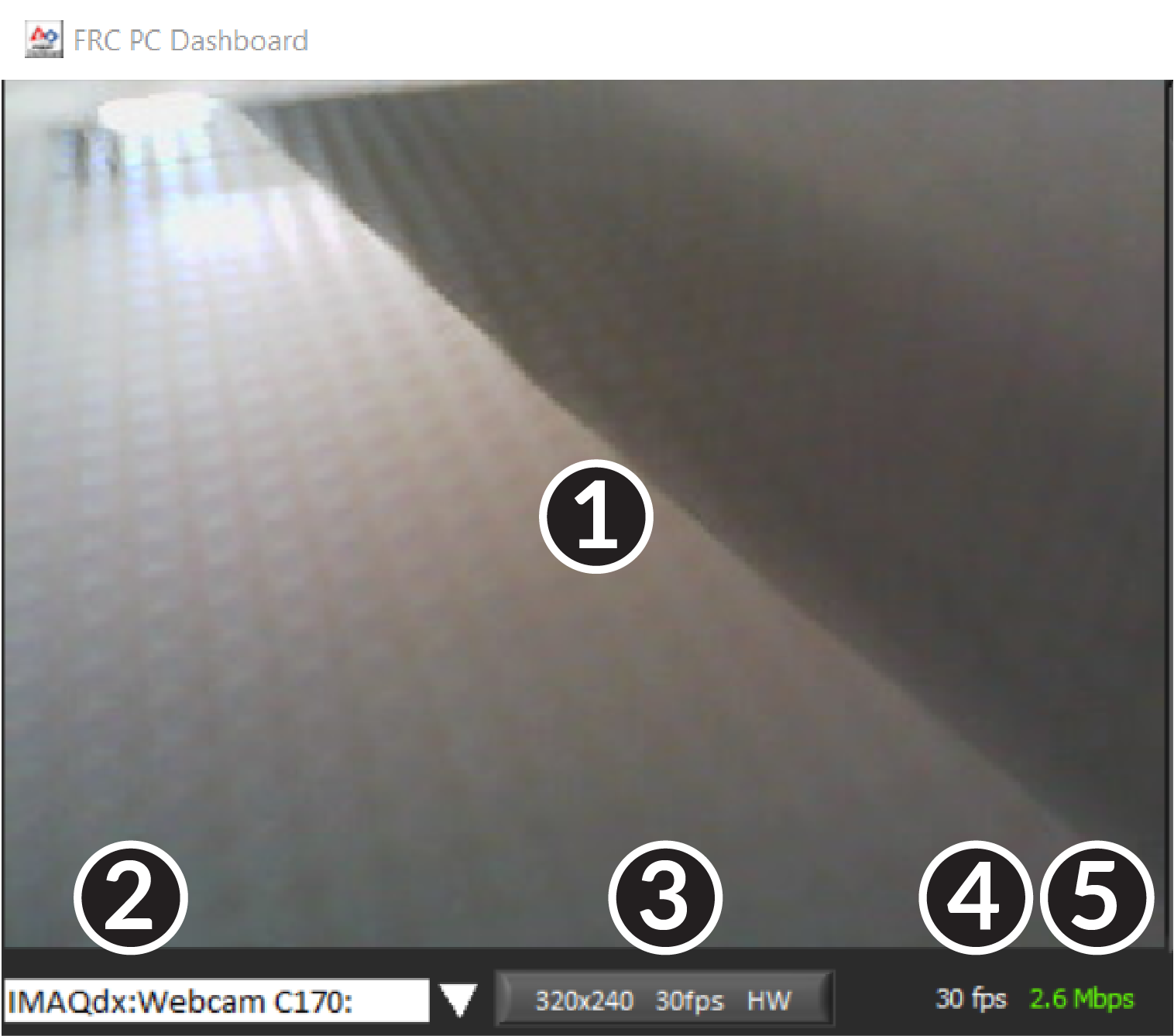
The left pane is used to display a video feed from an Axis camera or USB camera located on the robot. For instructions on setting up the Axis Camera to work with this display see here. There are also some controls and indicators related to the camera below the tab area:
Camera Image Display
Mode Selector - This drop-down allows you to select the type of camera display to use. The choices are Camera Off, USB Camera SW (software compression), USB Camera HW (hardware compression) and IP Camera (Axis camera). Note that the IP Camera setting will not work when your PC is connected to the roboRIO over USB.
Camera Settings - This control allows you to change the resolution, framerate and compression of the image stream to the dashboard, click the control to pop-up the configuration.
Bandwidth Indicator - Indicates approximate bandwidth usage of the image stream. The indicator will display green for “safe” bandwidth usage, yellow when teams should use caution and red if the stream bandwidth is beyond levels that will work on the competition field.
Framerate - Indicates the approximate received framerate of the image stream.
Tip
The bandwidth indicator indicates the combined bandwidth for all camera streams open.
Drive
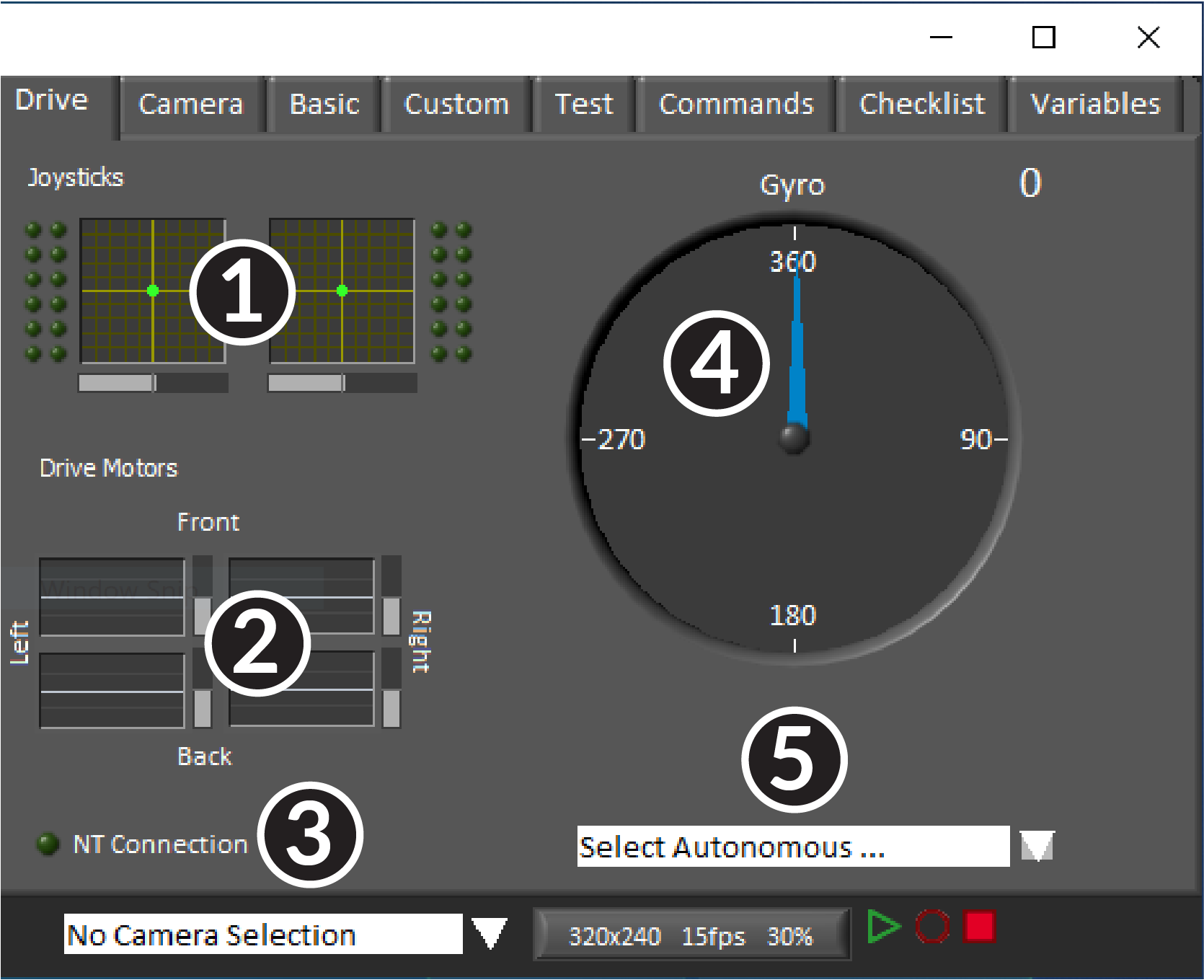
The center pane contains a section that provides feedback on the joysticks and drive commands when used with the LabVIEW framework and a section that displays the NetworkTables status and autonomous selector:
Displays X,Y and Throttle information and button values for up to 2 joysticks when using the LabVIEW framework
Displays values being sent to motor controllers when using LabVIEW framework
Displays a connection indicator for the NetworkTables data from the robot
Displays a Gyro value
Displays a text box that can be used to select Autonomous modes. Each language’s code templates have examples of using this box to select from multiple autonomous programs.
These indicators (other than the Gyro) are hooked up to appropriate values by default when using the LabVIEW framework. For information on using them with C++/Java code see Using the LabVIEW Dashboard with C++/Java Code.
Camera
Tip
The left pane can only display a single camera output, so use the camera tab on the right pane to display a second camera output if needed.
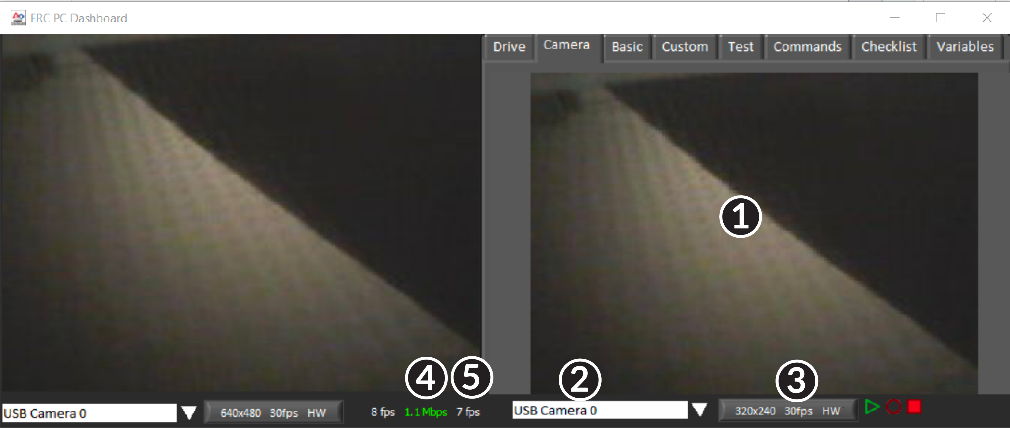
The camera tab is used to display a video feed from an Axis camera or USB camera located on the robot. For instructions on setting up the Axis Camera to work with this display see here. There are also some controls and indicators related to the camera below the tab area:
Camera Image Display
Mode Selector - This drop-down allows you to select the type of camera display to use. The choices are Camera Off, USB Camera SW (software compression), USB Camera HW (hardware compression) and IP Camera (Axis camera). Note that the IP Camera setting will not work when your PC is connected to the roboRIO over USB.
Camera Settings - This control allows you to change the resolution, framerate and compression of the image stream to the dashboard, click the control to pop-up the configuration.
Bandwidth Indicator - Indicates approximate bandwidth usage of the image stream. The indicator will display green for “safe” bandwidth usage, yellow when teams should use caution and red if the stream bandwidth is beyond levels that will work on the competition field.
Framerate - Indicates the approximate received framerate of the image stream.
Tip
The bandwidth indicator indicates the combined bandwidth for all camera streams open.
Basic
The Basic tab contains a variety of pre-populated bi-directional controls/indicators which can be used to control the robot or display information from the robot. The SmartDashboard key names associated with each item are labeled next to the indicator with the exception of the Strings which follow the same naming pattern and increment from DB/String 0 to DB/String 4 on the left and DB/String 5 to DB/String 9 on the right. The LabVIEW framework contains an example of reading from the Buttons and Sliders in Teleop. It also contains an example of customizing the labels in Begin. For more detail on using this tab with C++Java code, see Using the LabVIEW Dashboard with C++/Java Code.
Custom
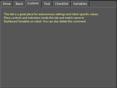
The Custom tab allows you to add additional controls/indicators to the dashboard using LabVIEW without removing any existing functionality. To customize this tab you will need to create a Dashboard project in LabVIEW.
Test
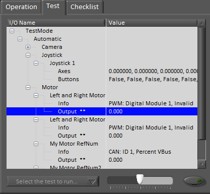
The Test tab is for use with Test mode for teams using LabVIEW (Java and C++ teams should use SmartDashboard or Shuffleboard when using Test Mode). For many items in the libraries, Input/Output info will be populated here automatically. All items which have ** next to them are outputs that can be controlled by the dashboard. To control an output, click on it to select it, drag the slider to set the value then press and hold the green button to enable the output. As soon as the green button is released, the output will be disabled. This tab can also be used to run and monitor tests on the robot. An example test is provided in the LabVIEW framework. Selecting this test from the dropdown box will show the status of the test in place of the slider and enable controls.
Commands
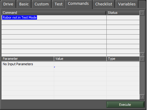
The Commands tab can be used with the Robot in Test mode to see which commands are running and to manually run commands for test purposes.
Checklist
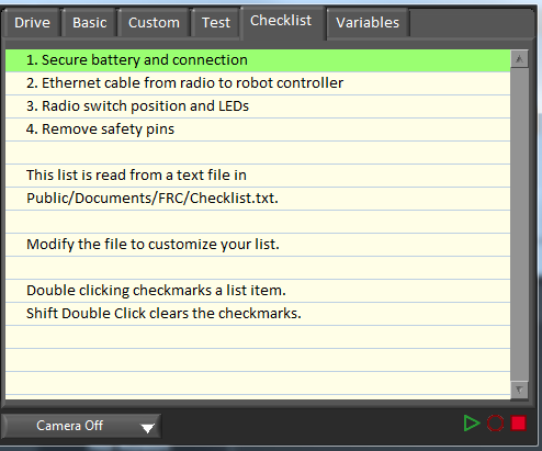
The Checklist tab can be used by teams to create a list of tasks to perform before or between matches. Instructions for using the Checklist tab are pre-populated in the default checklist file.
Variables
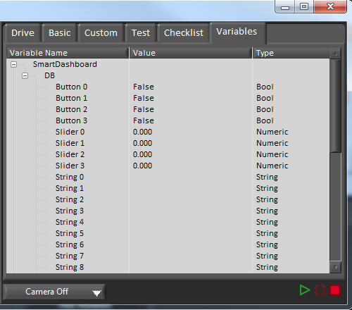
The Variables tab of the left pane shows all NetworkTables variables in a tree display. The Variable Name (Key), Value and data type are shown for each variable. Information about the NetworkTables bandwidth usage is also displayed in this tab. Entries will be shown with black diamonds if they are not currently synced with the robot.
Record/Playback
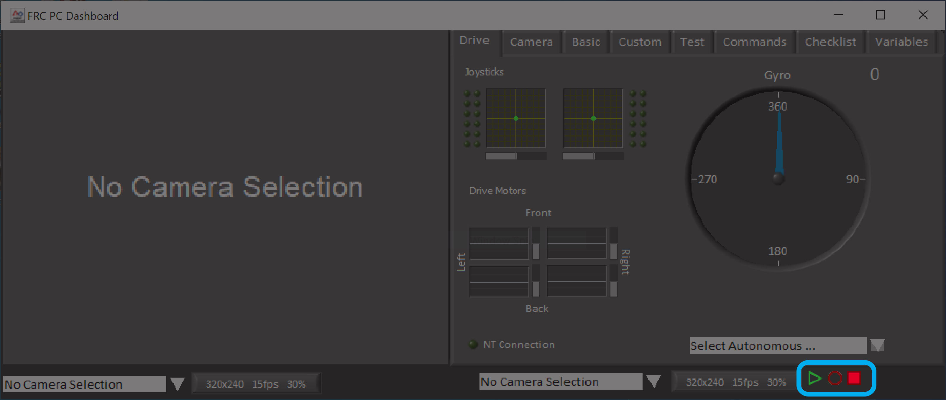
The LabVIEW Dashboard includes a Record/Playback feature that allows you to record video and NetworkTables data (such as the state of your Dashboard indicators) and play it back later.
Recording
To begin recording, click the red circular Record button. The background of the right pane will turn red to indicate you are recording. To stop recording, press the red square Stop button.
Playback
To play a recording back, click the green triangle Play button. The background of the right pane will begin pulsing green and playback controls will appear at the bottom of the camera pane.
File Selector - The dropdown allows you to select a log file to play back. The log files are named using the date and time and the dropdown will also indicate the length of the file. Selecting a logfile will immediately begin playing that file.
Play/Pause button - This button allows you to pause and resume playback of the log file.
Playback Speed - This dropdown allows you to adjust playback speed from 1/10 speed to 10x speed, the default is real-time (1x)
Time Control Slider - This slider allows you to fast-forward or rewind through the logfile by clicking on the desired location or dragging the slider.
Settings - With a log file selected, this dropdown allows you to rename or delete a file or open the folder containing the logs in Windows Explorer (Typically
C:\Users\Public\Documents\FRC\Log Files\Dashboard)
Using the LabVIEW Dashboard with C++/Java Code
The default LabVIEW Dashboard utilizes NetworkTables to pass values and is therefore compatible with C++ and Java robot programs. This article covers the keys and value ranges to use to work with the Dashboard.
Drive Tab
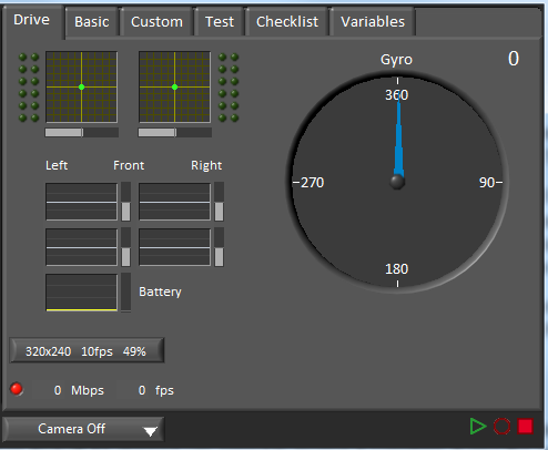
The Select Autonomous… dropdown can be used so show the available autonomous routines and choose one to run for the match.
SmartDashboard.putStringArray("Auto List", {"Drive Forwards", "Drive Backwards", "Shoot"});

// At the beginning of auto
String autoName = SmartDashboard.getString("Auto Selector", "Drive Forwards") // This would make "Drive Forwards the default auto
switch(autoName) {
   case "Drive Forwards":
     // auto here
   case "Drive Backwards":
     // auto here
   case "Shoot":
     // auto here
}
frc::SmartDashboard::PutStringArray("Auto List", {"Drive Forwards", "Drive Backwards", "Shoot"});

// At the beginning of auto
String autoName = SmartDashboard.GetString("Auto Selector", "Drive Forwards") // This would make "Drive Forwards the default auto
switch(autoName) {
   case "Drive Forwards":
     // auto here
   case "Drive Backwards":
     // auto here
   case "Shoot":
     // auto here
}
Sending to the “Gyro” NetworkTables entry will populate the gyro here.
SmartDashboard.putNumber("Gyro", drivetrain.getHeading());
frc::SmartDashboard::PutNumber("Gyro", Drivetrain.GetHeading());
There are four outputs that show the motor power to the drivetrain. This is configured for 2 motors per side and a tank style drivetrain. This is done by setting “RobotDrive Motors” like the example below.
SmartDashboard.putNumberArray("RobotDrive Motors", {drivetrain.getLeftFront(), drivetrain.getRightFront(), drivetrain.getLeftBack(), drivetrain.getRightBack()});
frc::SmartDashboard::PutNumberArray("Gyro", {drivetrain.GetLeftFront(), drivetrain.GetRightFront(), drivetrain.GetLeftBack(), drivetrain.GetRightBack()});
Basic Tab
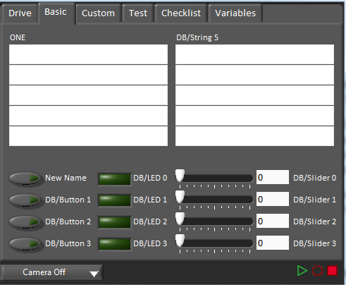
The Basic tab uses a number of keys in the a “DB” sub-table to send/receive Dashboard data. The LED’s are output only, the other fields are all bi-directional (send or receive).
Strings
The strings are labeled top-to-bottom, left-to-right from “DB/String 0” to “DB/String 9”. Each String field can display at least 21 characters (exact number depends on what characters). To write to these strings:
SmartDashboard.putString("DB/String 0", "My 21 Char TestString");
frc::SmartDashboard::PutString("DB/String 0", "My 21 Char TestString");
To read string data entered on the Dashboard:
String dashData = SmartDashboard.getString("DB/String 0", "myDefaultData");
std::string dashData = frc::SmartDashboard::GetString("DB/String 0", "myDefaultData");
Buttons and LEDs
The Buttons and LEDs are boolean values and are labeled top-to-bottom from “DB/Button 0” to “DB/Button 3” and “DB/LED 0” to “DB/LED 3”. The Buttons are bi-directional, the LEDs are only able to be written from the Robot and read on the Dashboard. To write to the Buttons or LEDs:
SmartDashboard.putBoolean("DB/Button 0", true);
frc::SmartDashboard::PutBoolean("DB/Button 0", true);
To read from the Buttons: (default value is false)
boolean buttonValue = SmartDashboard.getBoolean("DB/Button 0", false);
bool buttonValue = frc::SmartDashboard::GetBoolean("DB/Button 0", false);
Sliders
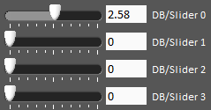
The Sliders are bi-directional analog (double) controls/indicators with a range from 0 to 5. To write to these indicators:
SmartDashboard.putNumber("DB/Slider 0", 2.58);
frc::SmartDashboard::PutNumber("DB/Slider 0", 2.58);
To read values from the Dashboard into the robot program: (default value of 0.0)
double dashData = SmartDashboard.getNumber("DB/Slider 0", 0.0);
double dashData = frc::SmartDashboard::GetNumber("DB/Slider 0", 0.0);
Troubleshooting Dashboard Connectivity
We have received a number of reports of Dashboard connectivity issues from events. This document will help explain how to recognize if the Dashboard is not connected to your robot, steps to troubleshoot this condition and a code modification you can make.
LabVIEW Dashboard
This section discusses connectivity between the robot and LabVIEW dashboard
Recognizing LabVIEW Dashboard Connectivity
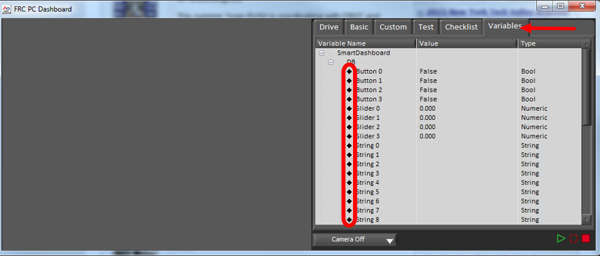
If you have an indicator on your dashboard that you expect to be changing it may be fairly trivial to recognize if the Dashboard is connected. If not, there is a way to check without making any changes to your robot code. On the Variables tab of the Dashboard, the variables are shown with a black diamond when they are not synced with the robot. Once the Dashboard connects to the robot and these variables are synced, the diamond will disappear.
Troubleshooting LabVIEW Dashboard Connectivity
If the Dashboard does not connect to the Robot (after the Driver Station has connected to the robot) the recommended troubleshooting steps are:
Close the Driver Station and Dashboard, then re-open the Driver Station (which should launch the Dashboard).
If that doesn’t work, restart the Robot Code using the Restart Robot Code button on the Diagnostics tab of the Driver Station
Recognizing Connectivity
This section discusses connectivity between the robot and SmartDashboard
Recognizing SmartDashboard Connectivity
The typical way to recognize connectivity with the SmartDashboard is to add a Connection Indicator widget and to make sure your code is writing at least one key during initialization or disabled to trigger the connection indicator. The connection indicator can be moved or re-sized if the Editable checkbox is checked.
Recognizing Shuffleboard Connectivity

Shuffleboard indicates if it is connected or not in the bottom right corner of the application as shown in the image above.
Recognizing Glass Connectivity
Glass displays if it is connected or not in the bar across the top. See this page for more on configuring the connection.
Troubleshooting Connectivity
If the Dashboard does not connect to the Robot (after the Driver Station has connected to the robot) the recommended troubleshooting steps are:
Restart the Dashboard (there is no need to restart the Driver Station software)
If that doesn’t work, restart the Robot Code using the Restart Robot Code button on the Diagnostics tab of the Driver Station
If it still doesn’t connect, verify that the Team Number / Server is set properly in the Dashboard and that your Robot Code writes a value during initialization or disabled
Telemetry
Telemetry: Recording Data on the Robot
Telemetry (literally “measuring remotely”) is the process of recording and sending real-time data about the performance of your robot to a real-time readout or log file. Recording and viewing telemetry data is a crucial part of the engineering process - accurate telemetry data helps you tune your robot to perform optimally, and is indispensable for debugging your robot when it fails to perform as expected.
Recording Data from Robot Code
Note
On-robot logging of telemetry data is not yet fully supported by WPILib (it is currently scheduled for a mid-season update). In the mean-time, teams can record their telemetry data on their driver station computer with Shuffleboard recordings.
WPILib supports several different ways to record and report telemetry data on the driver station.
At the most basic level, the Riolog provides support for viewing print statements from robot code. This is useful for on-the-fly debugging of problematic code, but does not scale as console interfaces are not suitable for rich data streams.
WPILib supports several dashboards that allow users to more easily send rich telemetry data to the driver-station computer. All WPILib dashboards communicate with the NetworkTables protocol, and so they are to some degree interoperable (telemetry logged with one dashboard will be visible on the others, but the specific widgets/formatting will generally not be compatible). NetworkTables (and thus WPILib all dashboards) currently support the following data types:
booleanboolean[]doubledouble[]stringstring[]byte[]
Telemetry data can be sent to a WPILib dashboard using an associated WPILib method (for more details, see the documentation for the individual dashboard in question), or by directly publishing to NetworkTables.
While NetworkTables does not yet support serialization of complex data types (this is tentatively scheduled for 2023), mutable types from user code can be easily extended to interface directly with WPILib dashboards via the Sendable interface, whose usage is described in the next article.
Robot Telemetry with Sendable
While the WPILib dashboard APIs allow users to easily send small pieces of data from their robot code to the dashboard, it is often tedious to manually write code for publishing telemetry values from the robot code’s operational logic.
A cleaner approach is to leverage the existing object-oriented structure of user code to declaratively mark important data fields for telemetry logging. The WPILib framework can then handle the tedious/tricky part of correctly reading from (and, potentially, writing to) those fields for you, greatly reducing the total amount of code the user has to write and improving readability.
WPILib provides this functionality with the Sendable interface. Classes that implement Sendable are able to register value listeners that automatically send data to the dashboard - and, in some cases, receive values back. These classes can be declaratively sent to any of the WPILib dashboards (as one would an ordinary data field), removing the need for teams to write their own code to send/poll for updates.
What is Sendable?
Sendable (Java, C++) is an interface provided by WPILib to facilitate robot telemetry. Classes that implement Sendable can declaratively send their state to the dashboard - once declared, WPILib will automatically send the telemetry values every robot loop. This removes the need for teams to handle the iteration-to-iteration logic of sending and receiving values from the dashboard, and also allows teams to separate their telemetry code from their robot logic.
Many WPILib classes (such as Commands) already implement Sendable, and so can be sent to the dashboard without any user modification. Users are also able to easily extend their own classes to implement Sendable.
The Sendable interface contains only one method: initSendable. Implementing classes override this method to perform the binding of in-code data values to structured JSON data, which is then automatically sent to the robot dashboard via NetworkTables. Implementation of the Sendable interface is discussed in the next article.
Sending a Sendable to the Dashboard
Note
Unlike simple data types, Sendables are automatically kept up-to-date on the dashboard by WPILib, without any further user code - “set it and forget it”. Accordingly, they should usually be sent to the dashboard in an initialization block or constructor, not in a periodic function.
To send a Sendable object to the dashboard, simply use the dashboard’s putData method. For example, an “arm” class that uses a PID Controller can automatically log telemetry from the controller by calling the following in its constructor:
SmartDashboard.putData("Arm PID", armPIDController);
frc::SmartDashboard::PutData("Arm PID", &armPIDController);
Additionally, some Sendable classes bind setters to the data values sent from the dashboard to the robot, allowing remote tuning of robot parameters.
Writing Your Own Sendable Classes
Since the Sendable interface only has one method, writing your own classes that implement Sendable (and thus automatically log values to and/or consume values from the dashboard) is extremely easy: just provide an implementation for the overrideable initSendable method, in which setters and getters for your class’s fields are declaratively bound to key values (their display names on the dashboard).
For example, here is the implementation of initSendable from WPILib’s BangBangController:
150  @Override
151  public void initSendable(SendableBuilder builder) {
152    builder.setSmartDashboardType("BangBangController");
153    builder.addDoubleProperty("tolerance", this::getTolerance, this::setTolerance);
154    builder.addDoubleProperty("setpoint", this::getSetpoint, this::setSetpoint);
155    builder.addDoubleProperty("measurement", this::getMeasurement, null);
156    builder.addDoubleProperty("error", this::getError, null);
157    builder.addBooleanProperty("atSetpoint", this::atSetpoint, null);
158  }
58void BangBangController::InitSendable(wpi::SendableBuilder& builder) {
59  builder.SetSmartDashboardType("BangBangController");
60  builder.AddDoubleProperty(
61      "tolerance", [this] { return GetTolerance(); },
62      [this](double tolerance) { SetTolerance(tolerance); });
63  builder.AddDoubleProperty(
64      "setpoint", [this] { return GetSetpoint(); },
65      [this](double setpoint) { SetSetpoint(setpoint); });
66  builder.AddDoubleProperty(
67      "measurement", [this] { return GetMeasurement(); }, nullptr);
68  builder.AddDoubleProperty(
69      "error", [this] { return GetError(); }, nullptr);
70  builder.AddBooleanProperty(
71      "atSetpoint", [this] { return AtSetpoint(); }, nullptr);
72}
To enable the automatic updating of values by WPILib “in the background”, Sendable data names are bound to getter and setter functions rather than specific data values. If a field that you wish to log has no defined setters and getters, they can be defined inline with a lambda expression.
The SendableBuilder Class
As seen above, the initSendable method takes a single parameter, builder, of type SendableBuilder (Java, C++). This builder exposes methods that allow binding of getters and setters to dashboard names, as well as methods for safely ensuring that values consumed from the dashboard do not cause unsafe robot behavior.
Databinding with addProperty Methods
Like all WPILib dashboard code, Sendable fields are ultimately transmitted over NetworkTables, and thus the databinding methods provided by SendableBuilder match the supported NetworkTables data types:
boolean:addBooleanPropertyboolean[]:addBooleanArrayPropertydouble:addDoublePropertydouble[]:addDoubleArrayPropertystring:addStringPropertystring[]:addStringArrayPropertybyte[]:addRawProperty
Ensuring Safety with setSafeState and setActuator
Since Sendable allows users to consume arbitrary values from the dashboard, it is possible for users to pipe dashboard controls directly to robot actuations. This is extremely unsafe if not done with care; dashboards are not a particularly good interface for controlling robot movement, and users generally do not expect the robot to move in response to a change on the dashboard.
To help users ensure safety when interfacing with dashboard values, SendableBuilder exposes a setSafeState method, which is called to place any Sendable mechanism that actuates based on dashboard input into a safe state. Any potentially hazardous user-written Sendable implementation should call setSafeState with a suitable safe state implementation. For example, here is the implementation from the WPILib PWMMotorController class:
118  @Override
119  public void initSendable(SendableBuilder builder) {
120    builder.setSmartDashboardType("Motor Controller");
121    builder.setActuator(true);
122    builder.setSafeState(this::disable);
123    builder.addDoubleProperty("Value", this::get, this::set);
124  }
54void PWMMotorController::InitSendable(wpi::SendableBuilder& builder) {
55  builder.SetSmartDashboardType("Motor Controller");
56  builder.SetActuator(true);
57  builder.SetSafeState([=] { Disable(); });
58  builder.AddDoubleProperty(
59      "Value", [=] { return Get(); }, [=](double value) { Set(value); });
60}
Additionally, users may call builder.setActuator(true) to mark any mechanism that might move as a result of Sendable input as an actuator. Currently, this is used by Shuffleboard to disable actuator widgets when not in LiveWindow mode.
Third-Party Telemetry Libraries
Tip
Is your library not listed here when it should be? Open a pull request to add it!
Several third-party logging utilities and frameworks exist that provide functionality beyond what is currently provided by WPILib:
AdvantageKit (Java only): “Log everything”-based logging framework with hooks for replaying logged data in simulation.
Oblog (Java only): Minimalistic annotation-based API for
Shuffleboard(or plainNetworkTables) telemetry.
FRC LabVIEW Programming
Creating Robot Programs
Tank Drive Tutorial
Question: How do I get my robot to drive with two joysticks using tank drive?
Solution: There are four components to consider when setting up tank drive for your robot. The first thing you will want to do is make sure the tank drive.vi is used instead of the arcade drive.vi or whichever drive VI you were utilizing previously. The second item to consider is how you want your joysticks to map to the direction you want to drive. In tank drive, the left joystick is used to control the left motors and the right joystick is used to control the right motors. For example, if you want to make your robot turn right by pushing up on the left joystick and down on the right joystick you will need to set your joystick’s accordingly in LabVIEW (this is shown in more detail below). Next, you will want to confirm the PWM lines that you are wired into, are the same ones your joysticks will be controlling. Lastly, make sure your motor controllers match the motor controllers specified in LabVIEW. The steps below will discuss these ideas in more detail:
Open LabVIEW and double click
FRC roboRIO Project.
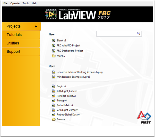
Give your project a name, add your team number, and select
Arcade Drive Robot roboRIO. You can select another option, however, this tutorial will discuss how to setup tank drive for this project.In the Project Explorer window, open up the
Robot Main.vi.Push Ctrl+E to see the block diagram. It should look like the following image:
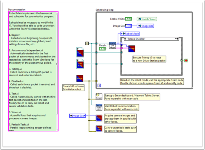
Double click the “Teleop” vi inside of the Teleop Enabled case structure. Look at its block diagram. You will want to make two changes here:
Replace Arcade Drive with the tank drive.vi. This can be found by right clicking on the block diagram >> WPI Robotics Library >> Robot Drive >> and clicking the Tank Drive VI.
Find the Index Array function that is after the Get Values.vi. You will need to create two numeric constants and wire each into one of the index inputs. You can determine what the values of each index should be by looking at the USB Devices tab in the FRC® Driver Station. Move the two joysticks to determine which number (index) they are tied to. You will likely want to use the Y-axis index for each joystick. This is because it is intuitive to push up on the joystick when you want the motors to go forward, and down when you when them to go in reverse. If you select the X-axis index for each, then you will have to move the joystick left or right (x-axis directions) to get the robot motors to move. In my setup, I’ve selected index 1 for my left motors Y-axis control and index 5 as the right motors Y-axis control. You can see the adjustments in LabVIEW in the following image:
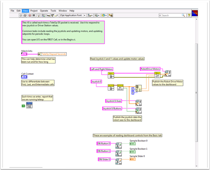
Next you will want to go back to your “Robot Main.vi” and double click on the “Begin.vi.”
The first thing to confirm in this VI is that your left and right motors are connected to the same PWM lines in LabVIEW as they are on your PDP (Power Distribution Panel).
The second thing to confirm in this VI is that the “Open 2 Motor.vi” has the correct motor controller selected (Talon, Jaguar, Victor, etc.).
For example, I am using Jaguar motor controllers and my motors are wired into PWM 8 and 9. The image below shows the changes I need to make:
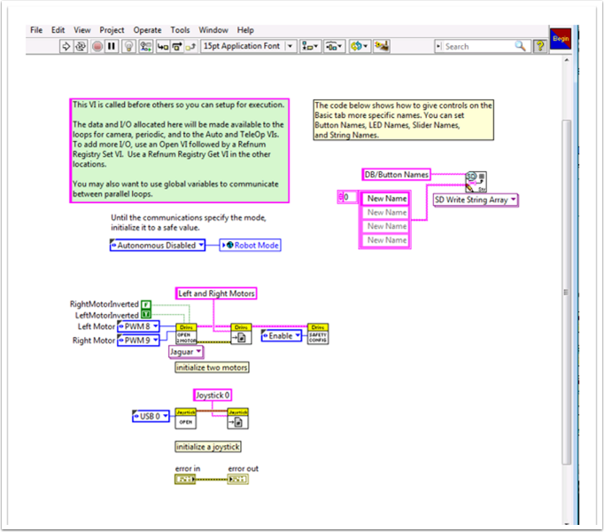
Save all of the Vis that you have made adjustments to and you are now able to drive a robot with tank drive!
Command and Control Tutorial
Introduction
Command and Control is a new LabVIEW template added for the 2016 season which organizes robot code into commands and controllers for a collection of robot-specific subsystems. Each subsystem has an independent control loop or state machine running at the appropriate rate for the mechanism and high-level commands that update desired operations and set points. This makes it very easy for autonomous code to build synchronous sequences of commands. Meanwhile, TeleOp benefits because it can use the same commands without needing to wait for completion, allowing for easy cancellation and initiation of new commands according to the drive team input. Each subsystem has a panel displaying its sensor and control values over time, and command tracing to aid in debugging.
What is Command and Control?
Command and Control recognizes that FRC® robots tend to be built up of relatively independent mechanisms such as Drive, Shooter, Arm, etc. Each of these is referred to as a subsystem and needs code that will coordinate the various sensors and actuators of the subsystem in order to complete requested commands, or actions, such as “Close Gripper” or “Lower Arm”. One of the key principles of this framework is that subsystems will each have an independent controller loop that is solely responsible for updating motors and other actuators. Code outside of the subsystem controller can issue commands which may change the robot’s output, but should not directly change any outputs. The difference is very subtle but this means that outputs can only possibly be updated from one location in the project. This speeds up debugging a robot behaving unexpectedly by giving you the ability to look through a list of commands sent to the subsystem rather than searching your project for where an output may have been modified. It also becomes easier to add an additional sensor, change gearing, or disable a mechanism without needing to modify code outside of the controller.
Game code, primarily consisting of Autonomous and TeleOp, will typically need to update set points and react to the state of certain mechanisms. For Autonomous, it is very common to define the robot’s operation as a sequence of operations – drive here, pick that up, carry it there, shoot it, etc. Commands can be wired sequentially with additional logic to quickly build complex routines. For teleOp, the same commands can execute asynchronously, allowing the robot to always process the latest driver inputs, and if implemented properly, new commands will interrupt, allowing the drive team to quickly respond to field conditions while also taking advantage of automated commands and command sequences.
Why should I use Command and Control?
Command and Control adds functionality to the existing LabVIEW project templates, allowing code to scale better with more sophisticated robots and robot code. Subsystems are used to abstract the details of the implementation, and game code is built from sequences of high level command VIs. The commands themselves are VIs that can update set points, perform numerical scaling/mapping between engineering units and mechanism units, and offer synchronization options. If physical changes are made to the robot, such as changing a gearing ratio, changes can be made to just a few command Vis to reflect this change across the entire code base.
I/O encapsulation makes for more predictable operation and quicker debugging when resource conflicts do occur. Because each command is a VI, you are able to single step through commands or use the built in Trace functionality to view a list of all commands sent to each subsystem.The framework uses asynchronous notification and consistent data propagation making it easy to program a sequence of commands or add in simple logic to determine the correct command to run.
Part 1: Project Explorer
The Project Explorer provides organization for all of the Vis and files you will use for your robot system. Below is a description of the major components in the Project Explorer to help with the expansion of our system. The most frequently used items have been marked in bold.
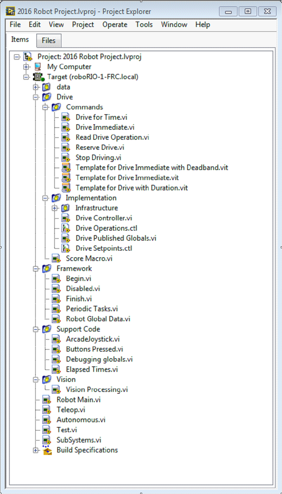
- My Computer
The items that define operation on the computer that the project was loaded on. For a robot project, this is used as a simulation target and is populated with simulation files.
- Sim Support Files
The folder containing 3D CAD models and description files for the simulated robot.
- Robot Simulation Readme.html
Documents the PWM channels and robot info you will need in order to write robot code that matches the wiring of the simulated robot.
- Dependencies
Shows the files used by the simulated robot’s code. This will populate when you designate the code for the simulated robot target.
- Build Specifications
This will contain the files that define how to build and deploy code for the simulated robot target.
- Target (roboRIO-TEAM-FRC.local)
The items that define operation on the roboRIO located at (address).
- Drive
The subsystem implementation and commands for the robot drive base. This serves as a custom replacement for the WPILib RobotDrive VIs.
- Framework
VIs used for robot code that is not part of a subsystem that are not used very often.
- Begin
Called once when robot code first starts. This is useful for initialization code that doesn’t belong to a particular subsystem.
- Disabled
Called once for each disabled packet and can be used to debug sensors when you don’t want the robot to move.
- Finish
During development, this may be called when robot code finishes. Not called on abort or when power is turned off.
- Periodic Tasks
A good place for ad hoc periodic loops for debugging or monitoring
- Robot Global Data
Useful for sharing robot information that doesn’t belong to a subsystem.
- Support Code
Debugging and code development aids.
- Vision
Subsystem and commands for the camera and image processing.
- Robot Main.vi
Top level VI that you will run while developing code.
- Autonomous.vi
VI that runs during autonomous period.
- Teleop.vi
VI that is called for each TeleOp packet.
- Test.vi
VI that runs when driver station is in test mode.
- SubSystems.vi
VI that contains and starts all subsystems.
- Dependencies
Shows the files used by the robot code.
- Build Specifications
Used to build and run the code as a startup application once code works correctly.
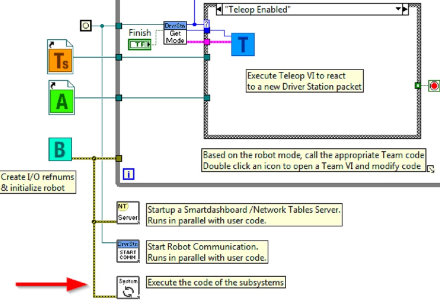
Drive Subsystem Project Explorer
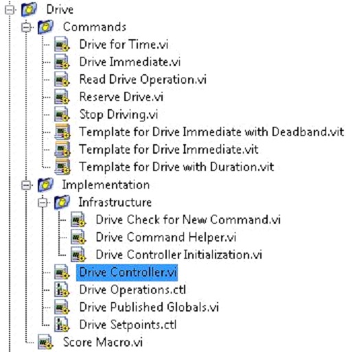
- Commands:
This folder contains the command VIs that request the controller carry out an operation. It also contains templates for creating additional drive commands.
Note
After creating a new command, you may need to edit Drive Setpoints.ctl to add or update fields that controller uses to define the new operation. You also need to go into the Drive Controller.vi and modify the case structure to add a case for every value.
Implementation
These are the VIs and Controls used to build the subsystem.
- Infrastructure VIs
Drive Check for New Command: It is called each iteration of the controller loop. It checks for new commands, updates timing data, and upon completion notifies a waiting command.
Drive Command Helper.vi: Commands call this VI to notify the controller that a new command has been issued.
Drive Controller Initialization.vi: It allocates the notifier and combines the timing, default command, and other information into a single data wire.
Drive Controller.vi: This VI contains the control/state machine loop. The panel may also contain displays useful for debugging.
Drive Operation.ctl: This typedef defines the operational modes of the controller. Many commands can share an operation.
Drive Setpoint.ctl: It contains the data fields used by all operating modes of the Drive subsystem.
Drive Published Globals.vi: A useful place for publishing global information about the drive subsystem.
Part 2: Initializing the Drive Subsystem
There are green comments on the controller’s block diagram that point out key areas that you will want to know how to edit.
The area to the left of the control loop will execute once when the subsystem starts up. This is where you will typically allocate and initialize all I/O and state data. You may publish the I/O refnums, or you may register them for Test Mode Only to keep them private so that other code cannot update motors without using a command.
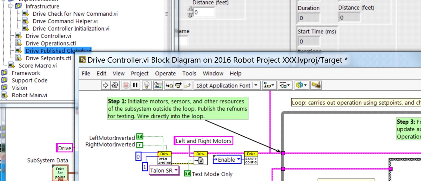
Note
Initializing the resources for each subsystem in their respective Controller.vi rather than in Begin.vi improves I/O encapsulation, reducing potential resource conflicts and simplifies debugging.
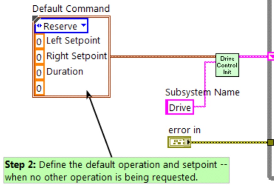
Part of the initialization is to select the default operation and set point values when no other operation is being processed.
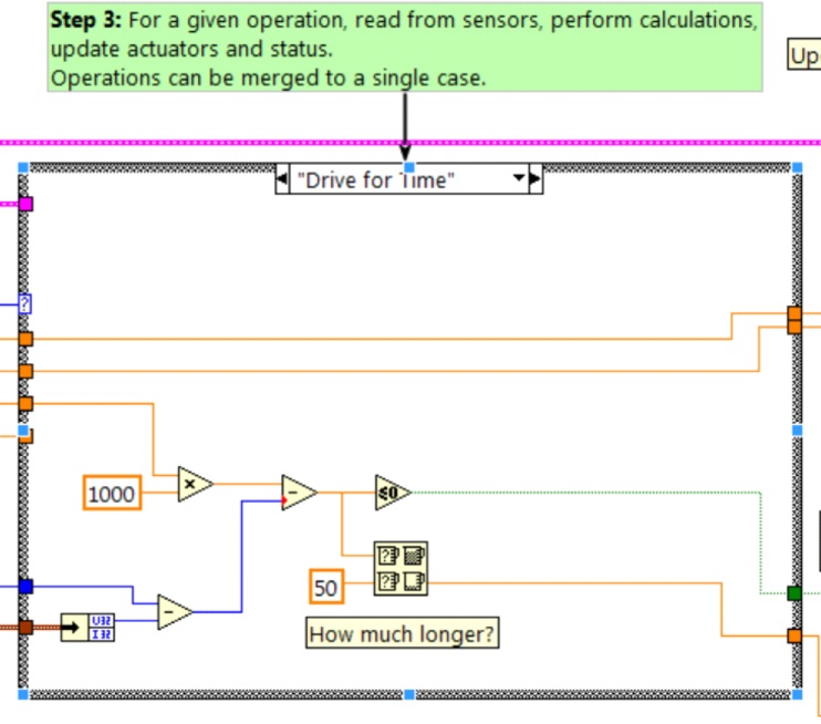
Inside the control loop is a case statement where operations are actually implemented. Set point values, iteration delay, iteration count, and sensors can all have influence on how the subsystem operates. This case structure has a value for each operation state of the subsystem.
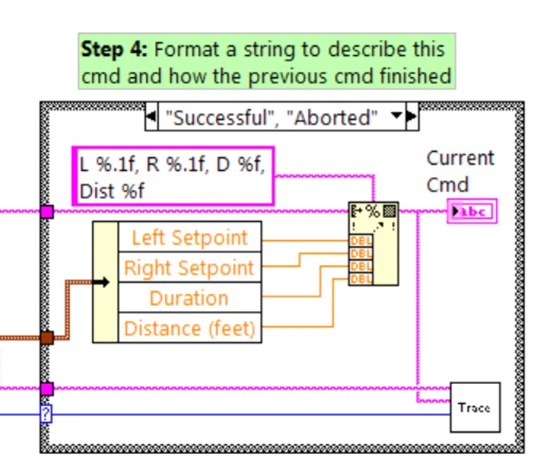
Each iteration of the controller loop will optionally update the Trace VI. The framework already incorporates the subsystem name, operation, and description, and you may find it helpful to format additional set point values into the trace information. Open the Trace VI and click Enable while the robot code is running to current setpoints and commands sent to each subsystem.
The primary goal of the controller is to update actuators for the subsystem. This can occur within the case structure, but many times, it is beneficial to do it downstream of the structure to ensure that values are always updated with the correct value and in only one location in the code.
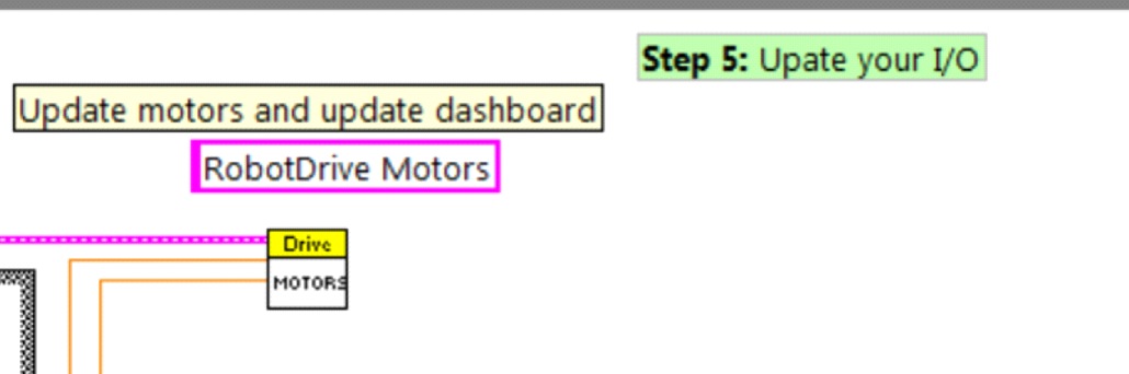
Part 3: Drive Subsystem Shipped Commands
There are 3 shipped example commands for each new subsystem:
Drive For Time.vi

This VI sets the motors to run for a given number of seconds. It optionally synchronizes with the completion of the command.
The Drive for Time case will operate the motors at the set point until the timer elapses or a new command is issued. If the motors have the safety timeout enabled, it is necessary to update the motors at least once every 100ms. This is why the code waits for the smaller of the remaining time and 50ms.
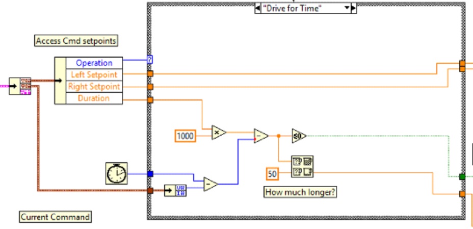
Drive Immediate.vi

Gets the desired left and right speeds for the motors and will set the motors immediately to those set points.
The Immediate case updates the motors to the set point defined by the command. The command is not considered finished since you want the motors to maintain this value until a new command comes in or until a timeout value. The timeout is useful anytime a command includes a dead band. Small values will not be requested if smaller than the dead band, and will result in growling or creeping unless the command times out.
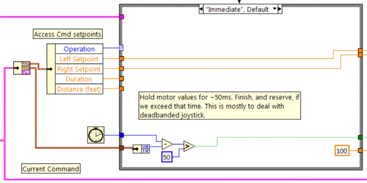
Stop Driving.vi

Zero the drive motors, making the robot stationary.
The Reserve command turns off the motors and waits for a new command. When used with a named command sequence, reserve identifies that the drive subsystem is part of a sequence, even if not currently moving the robot. This helps to arbitrate subsystem resource between simultaneously running commands.
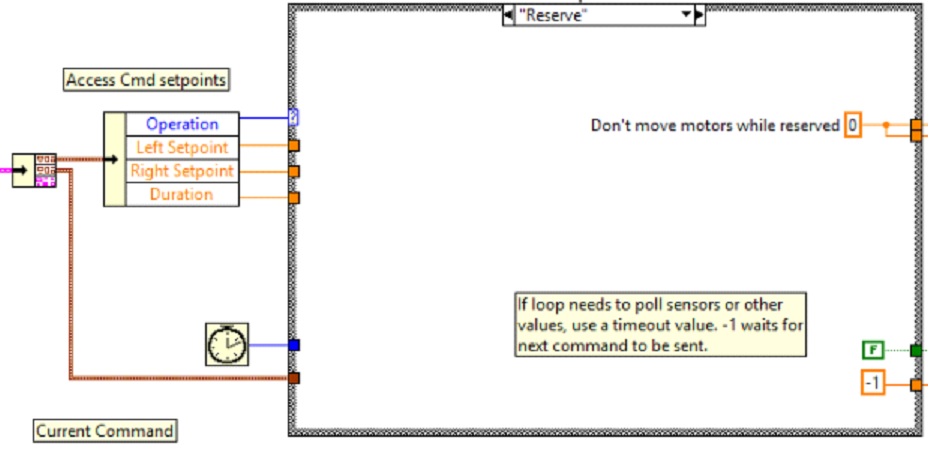
Part 4: Creating New Commands
The Command and Control framework allows users to easily create new commands for a subsystem. To Create a new command open the subsystem folder/Commands In the project explorer window, choose one of the VI Templates to use as the starting point of your new command, right click, and select New From Template.
Immediate: This VI notifies the subsystem about the new setpoint.
Immediate with deadband: This VI compares the input value to the deadband and optionally notifies the subsystem about the new setpoint. This is very useful when joystick continuous values are being used.
With duration: This VI notifies the subsystem to perform this command for the given duration, and then return to the default state. Synchronization determines whether this VI Starts the operation and returns immediately, or waits for the operation to complete. The first option is commonly used for TeleOp, and the second for Autonomous sequencing.
In this example we will add the new command “Drive for Distance”.
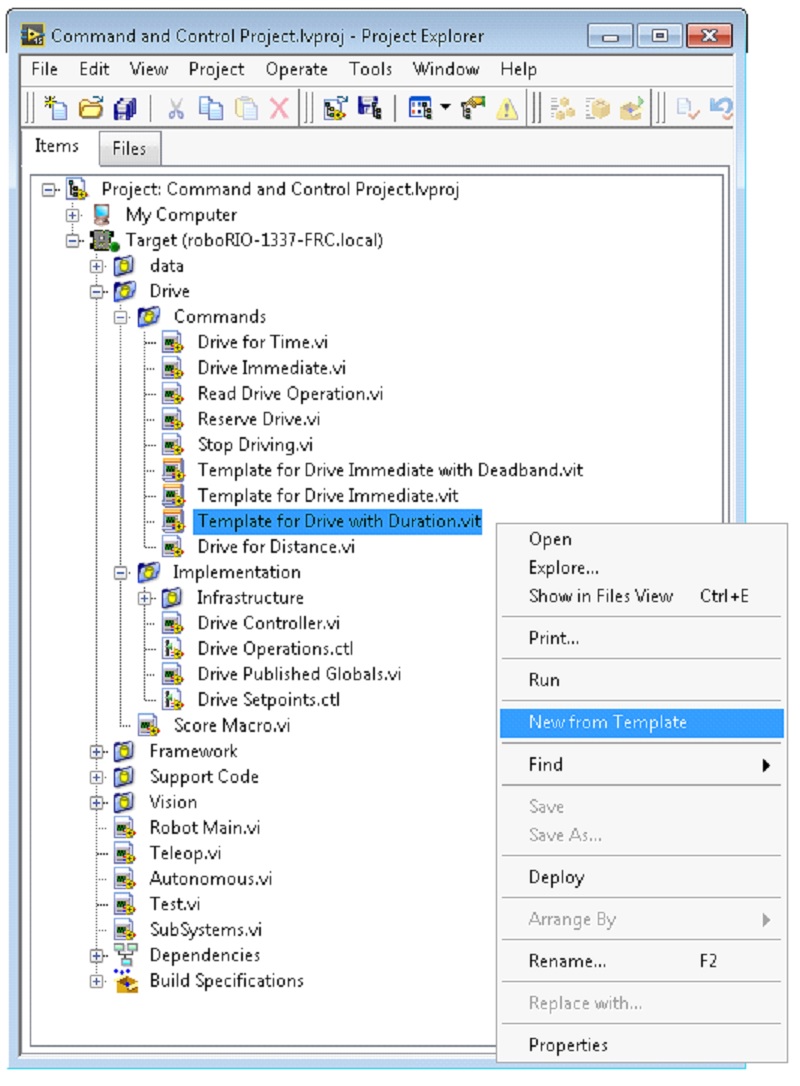
First, save the new VI with a descriptive name such as “Drive for Distance”. Next, determine whether the new command needs a new value added the Drive Operations enum typedef. The initial project code already has an enum value of Drive for Distance, but the following image shows how you would add one if needed.
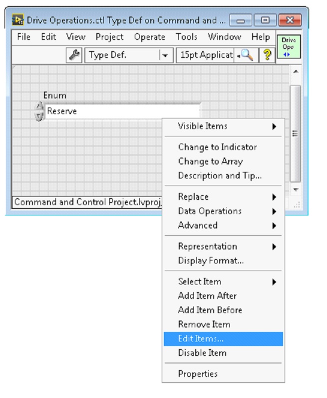
If a command needs additional information to execute, add it to the setpoints control. By default, the Drive subsystem has fields for the Left Setpoint, Right Setpoint, and Duration along with the operation to be executed. The Drive for Distance command could reuse Duration as distance, but let’s go ahead and add a numeric control to the Drive Setpoints.ctl called Distance (feet).
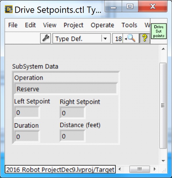
Once that we have all of the fields needed to specify our command, we can modify the newly created Drive for Distance.vi. As shown below, select Drive for Distance from the enum’s drop down menu and add a VI parameters to specify distance, speeds, etc. If the units do not match, the command VI is a great place to map between units.
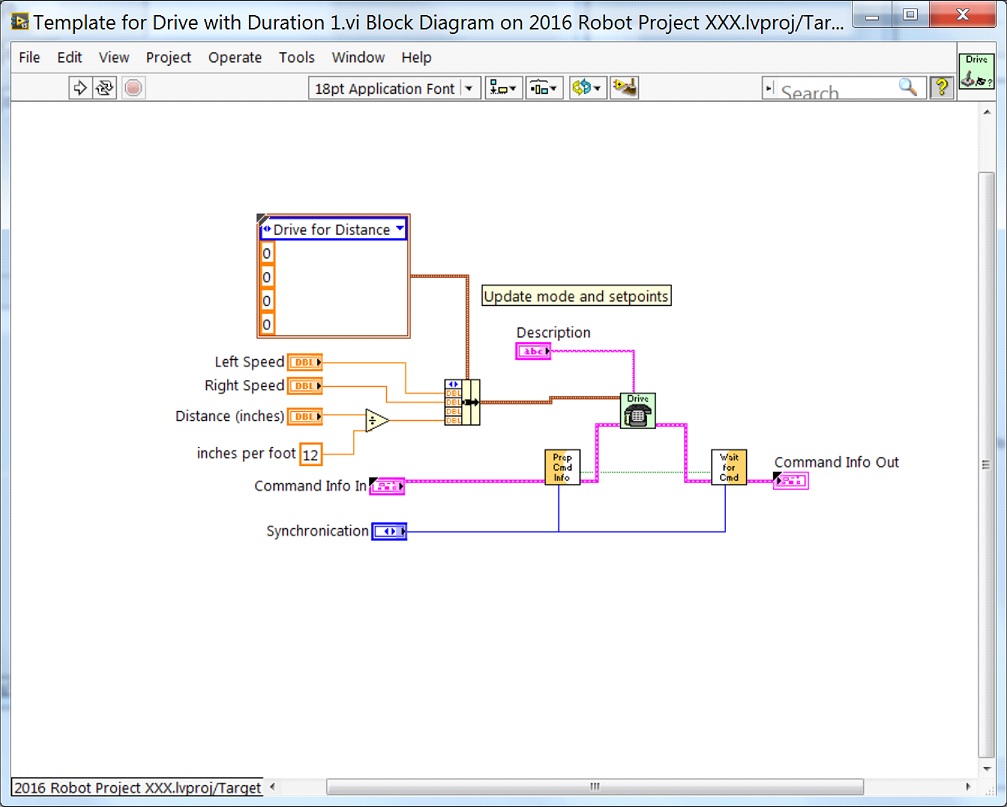
Next, add code to the Drive Controller to define what happens when the Drive for Distance command executes. Right click on the Case Structure and Duplicate or Add Case for Every Value. This will create a new “Drive for Distance” case.
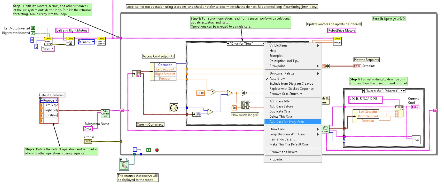
In order to access new setpoint fields, grow the “Access Cmd setpoints” unbundle node. Open your encoder(s) on the outside, to the left of the loop. In the new diagram of the case structure, we added a call to reset the encoder on the first loop iteration and read it otherwise. There is also some simple code that compares encoder values and updates the motor power. If new controls are added to the setpoints cluster, you should also consider adding them to the Trace. The necessary changes are shown in the image below.
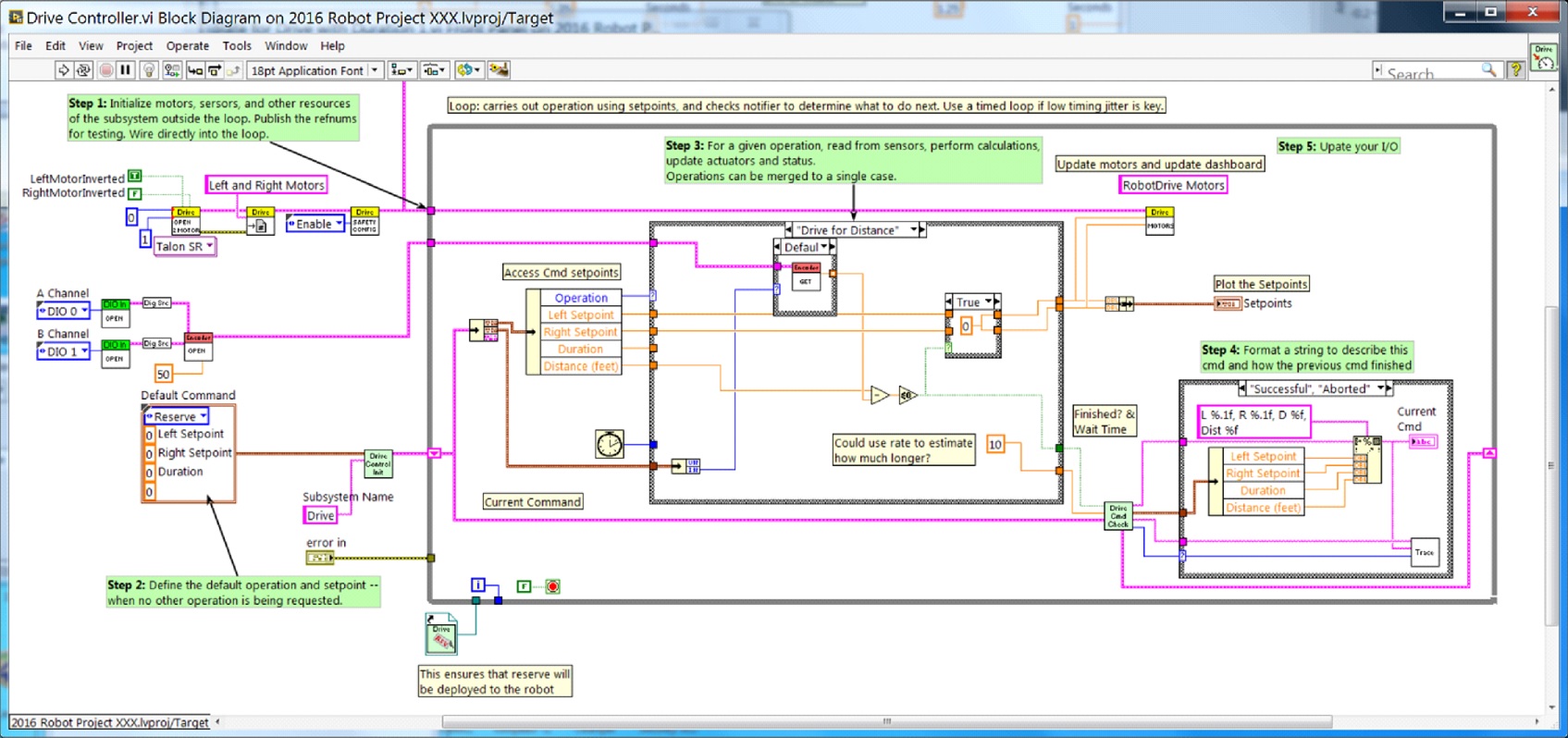
Part 5: Creating a Subsystem
In order to create a new subsystem, right click on the roboRIO target and select New» Subsystem. In the pop up dialog box, enter the name of the subsystem, list the operational modes, and specify the color of the icon.
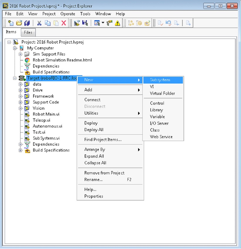
When you click OK, the subsystem folder will be generated and added to the project disk folder and tree. It will contain a base implementation of the VIs and controls that make up a subsystem. A call to the new controller will be inserted into the Subsystems VI. The controller VI will open, ready for you to add I/O and implement state machine or control code. Generated VI icons will use the color and name provided in the dialog. The generated code will use typedefs for set point fields and operations.
Below is the block diagram of the newly created subsystem. This code will be generated automatically when you create the subsystem.
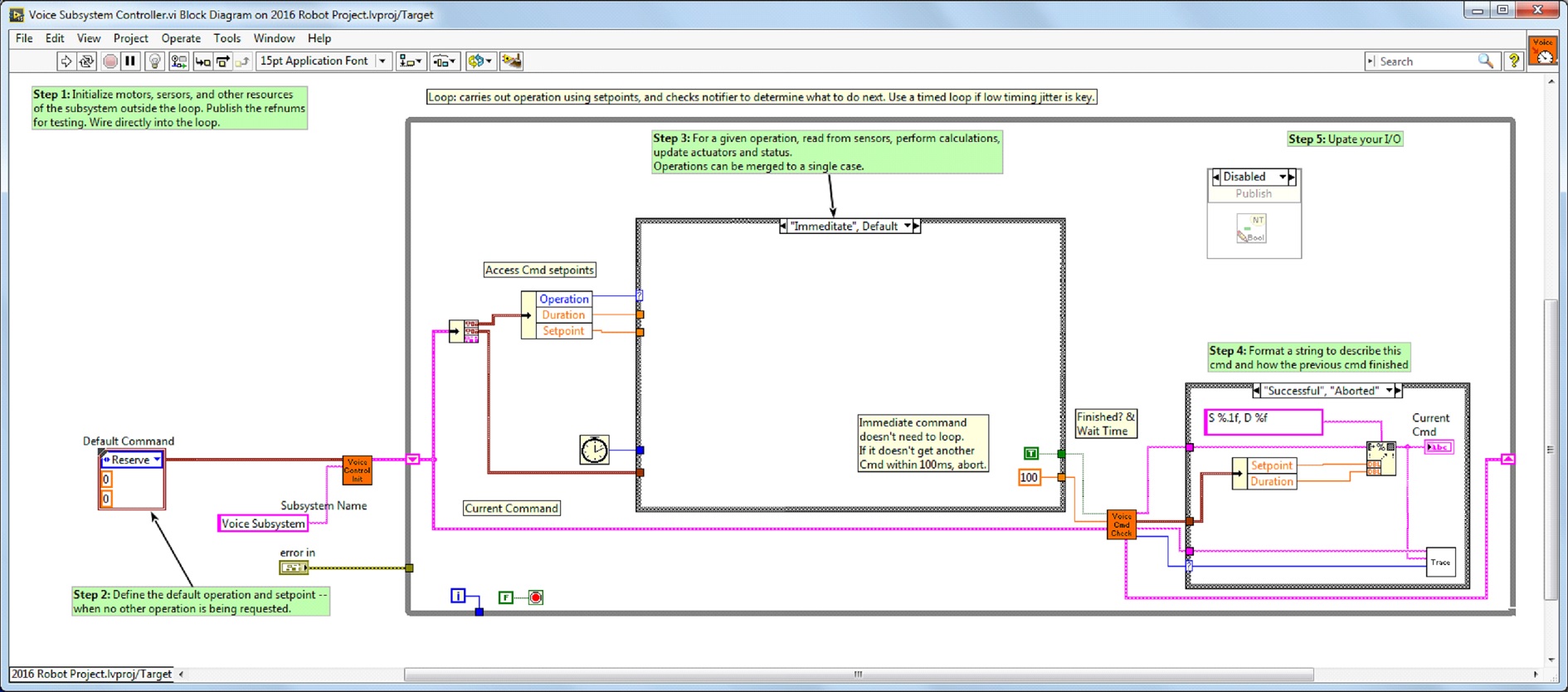
LabVIEW Resources
LabVIEW Resources
Note
To learn more about programming in LabVIEW and specifically programming FRC® robots in LabVIEW, check out the following resources.
LabVIEW Basics
NI provides tutorials on the basics of LabVIEW. These tutorials can help you get acquainted with the LabVIEW environment and the basics of the graphical, dataflow programing model used in LabVIEW.
NI FRC Tutorials
NI also hosts many FRC specific tutorials and presentations ranging from basic to advanced. For an in-depth single resource check out the FRC Basic and Advanced Training Classes linked near the bottom of the page.
Installed Tutorials and Examples
There are also tutorials and examples for all sorts of tasks and components provided as part of your LabVIEW installation. To access the tutorials, from the LabVIEW Splash screen (the screen that appears when the program is first launched) click on the Tutorials tab on the left side. Note that the tutorials are all in one document, so once it is open you are free to browse to other tutorials without returning to the splash screen.
To access the examples either click the Support tab, then Find FRC Examples or anytime you’re working on a program open the Help menu, select Find Examples and open the FRC Robotics folder.
Waiting for Target to Respond - Recovering from bad loops
Note
If you download LabVIEW code which contains an unconstrained loop (a loop with no delay) it is possible to get the roboRIO into a state where LabVIEW is unable to connect to download new code. This document explains the process required to load new, fixed, code to recover from this state.waiting-for-target-to-respond/
The Symptom
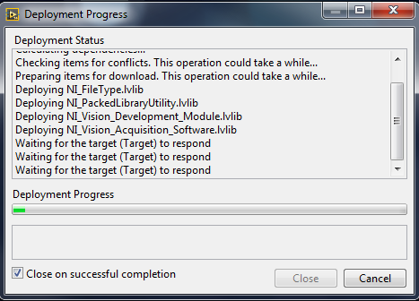
The primary symptom of this issue is attempts to download new robot code hang at the “Waiting for the target (Target) to respond” step as shown above. Note that there are other possible causes of this symptom (such as switching from a C++Java program to LabVIEW program) but the steps described here should resolve most or all of them.
Click Cancel to close the download dialog.
The Problem
One common source of this issue is unconstrained loops in your LabVIEW code. An unconstrained loop is a loop which does not contain any delay element (such as the one on the left). If you are unsure where to begin looking, Disabled.VI, Periodic Tasks.VI and Vision Processing.VI are the common locations for this type of loop. To fix the issue with the code, add a delay element such as the Wait (ms) VI from the Timing palette, found in the right loop.
Set No App

Using the roboRIO webserver (see the article on the roboRIO Web Dashboard Startup Settings for more details). Check the box to “Disable RT Startup App”.
Reboot
Reboot the roboRIO, either using the Reset button on the device or by click Restart in the top right corner of the webpage.
Clear No App
Using the roboRIO webserver (see the article on the roboRIO Web Dashboard Startup Settings for more details). Uncheck the box to “Disable RT Startup App”.
Load LabVIEW Code
Load LabVIEW code (either using the Run button or Run as Startup). Make sure to set LabVIEW code to Run as Startup before rebooting the roboRIO or you will need to follow the instructions above again.
How To Toggle Between Two Camera Modes
This code shows how to use a button to toggle between two distinct camera modes. The code consists of four stages.
In the first stage, the value of a button on the joystick is read.
Next, the current reading is compared to the previous reading using a Feedback Node and some Boolean arithmetic. Together, these ensure that the camera mode is only toggled when the button is initially pressed rather than toggling back and forth multiple times while the button is held down.
After that, the camera mode is toggled by masking the result of the second stage over the current camera mode value. This is called bit masking and by doing it with the XOR function the code will toggle the camera mode when the second stage returns true and do nothing otherwise.
Finally, you can insert the code for each camera mode in the case structure at the end. Each time the code is run, this section will run the code for the current camera mode.
LabVIEW Examples and Tutorials
Popular Tutorials
Autonomous Timed Movement Tutorial
Move your robot autonomously based on different time intervals
Setup your roboRIO motor hardware and software
Learn to setup the FRC® Control System and FRC Robot Project
Learn basic Image Processing techniques and how to use NI Vision Assistant
What is PID Control and how can I implement it?
What is Command and Control?
How do I implement it?
Get to know the FRC Driver Station
Learn to setup and use Test Mode
Looking for more examples and discussions? Search through more documents or post your own discussion, example code, or tutorial by clicking here! Don’t forget to mark your posts with a tag!
Add an Independent Motor to a Project
Once your drive that controls the wheels is all set, you might need to add an additional motor to control something completely independent of the wheels, such as an arm. Since this motor will not be part of your tank, arcade, or mecanum drive, you’ll definitely want independent control of it.
These VI Snippets show how to set up a single motor in a project that may already contain a multi-motor drive. If you see the HAND>ARROW>LABVIEW symbol, just drag the image into your block diagram, and voila: code! Ok, here’s how you do it.
FIRST, create a motor reference in the Begin.vi, using the Motor Control Open VI and Motor Control Refnum Registry Set VI. These can be found by right-clicking in the block diagram and going to WPI Robotics Library>>RobotDrive>>Motor Control. Choose your PWM line and name your motor. I named mine “Lift Motor” and connected it to PWM 7. (I also included and enabled the Motor Control Safety Config VI, which automatically turns off the motor if it loses connection.)
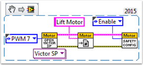
Now, reference your motor (the name has to be exact) in the Teleop.vi using the Motor Control Refnum Registry Get VI and tell it what to do with the Motor Control Set Output VI. These are in the same place as the above VIs.
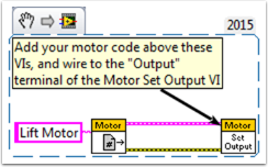
For example, the next snippet tells the Lift Motor to move forward if button 4 is pressed on Joystick 0 and to remain motionless otherwise. For me, button 4 is the left bumper on my Xbox style controller (“Joystick 0”). For much more in-depth joystick button options, check out How to Use Joystick Buttons to Control Motors or Solenoids.
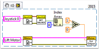
Finally, we need to close the references in the Finish.vi (just like we do with the drive and joystick), using the Motor Control Refnum Registry Get VI and Motor Control Close VI. While this picture shows the Close VI in a flat sequence structure by itself, we really want all of the Close VIs in the same frame. You can just put these two VIs below the other Get VIs and Close VIs (for the joystick and drive).
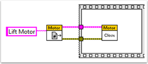
I hope this helps you program the best robot ever! Good luck!
Keyboard Navigation with the roboRIO
This example provides some suggestions for controlling the robot using keyboard navigation in place of a joystick or other controller. In this case, we use the A, W, S, and D keys to control two drive motors in a tank drive configuration.
The first VI Snippet is the code that will need to be included in the Dashboard Main VI. You can insert this code into the True case of Loop 1. The code opens a connection to the keyboard before the loop begins, and on each iteration it reads the pressed key. This information is converted to a string, which is then passed to the Teleop VI in the robot project. When Loop 1 stops running, the connection to the keyboard is closed.
The second VI Snippet is code that should be included in the Teleop VI. This reads the string value from the Dashboard that indicates which key was pressed. A Case Structure then determines which values should be written to the left and right motors, depending on the key. In this case, W is forward, A is left, D is right, and S is reverse. Each case in this example runs the motors at half speed. You can keep this the same in your code, change the values, or add additional code to allow the driver to adjust the speed, so you can drive fast or slow as necessary. Once the motor values are selected, they are written to the drive motors, and motor values are published to the dashboard.
Making a One-Shot Button Press
When using the Joystick Get Values function, pushing a joystick button will cause the button to read TRUE until the button is released. This means that you will most likely read multiple TRUE values for each press. What if you want to read only one TRUE value each time the button is pressed? This is often called a “One-Shot Button”. The following tutorial will show you how to create a subVI that you can drop into your Teleop.vi to do this.
First, create a new VI in the Support Code folder of your project.
Now on the block diagram of the new VI, drop in the following code snippet.
This code uses a function called the Feedback Node. We have wired the current value of the button into the left side of the feedback node. The wire coming out of the arrow of the feedback node represents the previous value of the button. If the arrow on your feedback node is going the opposite direction as shown here, right click to find the option to reverse the direction.
When a button is pressed, the value of the button goes from FALSE to TRUE. We want the output of this VI to be TRUE only when the current value of the button is TRUE, and the previous value of the button is FALSE.
Next we need to connect the boolean control and indicator to the inputs and outputs of the VI. To do this, first click the block on the connector pane, then click the button to connect the two (see the diagram below). Repeat this for the indicator.
Next, we need to change the properties of this VI so that we can use multiples of this VI in our TeleOp.vi. Right click the VI Icon and go to VI Properties. Then select the category “Execution” and select “Preallocated clone reentrant execution”.
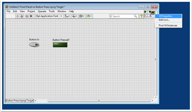
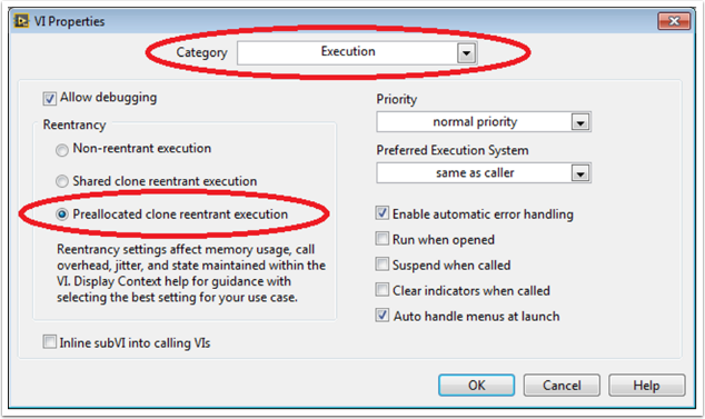
Lastly, we should change the VI Icon to be more descriptive of the VI’s function. Right click the Icon and go to Edit Icon. Create a new Icon.
Finally, save the VI with a descriptive name. You can now drag and drop this VI from the Support Files folder into your TeleOp.vi. Here is a copy of the completed VI: Button_Press.vi
Here’s an example of how you could use this VI.
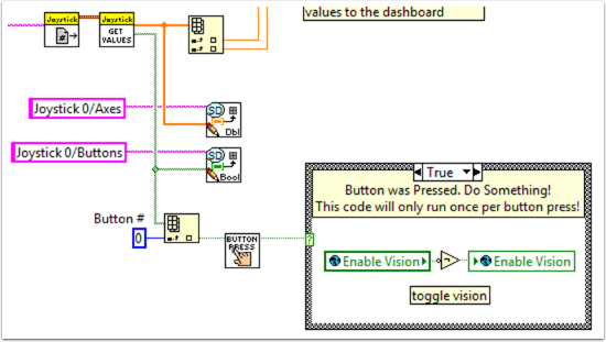
Adding Safety Features to Your Robot Code
A common problem with complex projects is making sure that all of your code is executing when you expect it to. Problems can arise when tasks with high priority, long execution times, or frequent calls hog processing power on the roboRIO. This leads to what is known as “starvation” for the tasks that are not able to execute due to the processor being busy. In most cases this will simply slow the reaction time to your input from the joysticks and other devices. However, this can also cause the drive motors of your robot to stay on long after you try to stop them. To avoid any robotic catastrophes from this, you can implement safety features that check for task input starvation and automatically shut down potentially harmful operations.
There are built-in functions for the motors that allow easy implementation of safety checks. These functions are:
Robot Drive Safety Configuration
Motor Drive Safety Configuration
Relay Safety Configuration
PWM Safety Configuration
Solenoid Safety Configuration
Robot Drive Delay and Update Safety
In all of the Safety Configuration functions, you can enable and disable the safety checks while your programming is running and configure what timeout you think is appropriate. The functions keep a cache of all devices that have the safety enabled and will check if any of them have exceeded their time limit. If any has, all devices in the cache will be disabled and the robot will come to an immediate stop or have its relay/PWM/solenoid outputs turned off. The code below demonstrates how to use the Drive Safety Configuration functions to set a maximum time limit that the motors will receive no input before being shut off.
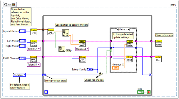
To test the safety shut-off, try adding a Wait function to the loop that is longer than your timeout!
The final function that relates to implementing safety checks–Robot Drive Delay and Update Safety–allows you to put the roboRIO in Autonomous Mode without exceeding the time limit. It will maintain the current motor output without making costly calls to the Drive Output functions, and will also make sure that the safety checks are regularly updated so that the motors will not suddenly stop.
Overall, it is highly recommended that some sort of safety check is implemented in your project to make sure that your robot is not unintentionally left in a dangerous state!
How to Use Joystick Buttons to Control Motors or Solenoids
As we all get our drive systems working, we are moving on to connecting our auxiliary devices such as motors and solenoids. With this, we will generally use joystick buttons to control these devices. To get started with this, we’ll go through several ways to control devices with joystick buttons.
Did you know that you can click and drag a VI Snippet from a document like this right into your LabVIEW code? Try it with the snippets in this document.
Setup:
No matter what the configuration, you’ll need to add one, two, or more (if you’re really excited) joysticks to the “Begin.vi”. The first example uses 2 joysticks and the others only use one. Give each one a unique name so we can use it in other places, like the snippet below. I named them “LeftStick” and “RightStick” because they are on the left and right sides of my desk. If your joysticks are already configured, great! You can skip this step.
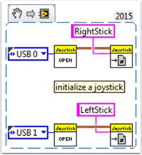
The rest of the code in this document will be placed in the “Teleop.VI” This is where we will be programming our joystick buttons to control different aspects of our motors or solenoids.
Scenario 1
“I want a motor to move one way when I press one button and the other way when I press a different button.”
This code uses button 0 on two different joysticks to control the same motor. If button 0 on LeftStick is pressed, the motor moves backward, and if button 0 on RightStick is pressed, the motor moves forward. If both buttons are pressed or neither button is pressed, the motor doesn’t move. Here I named my motor reference “Motor5”, but you can name your motor whatever you want in the “Begin.vi”
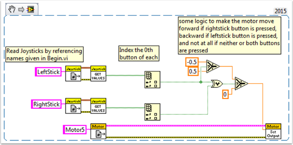
You may want to use multiple buttons from the same joystick for control. For an example of this, look at the following VI snippet or the VI snippet in Scenario 2.
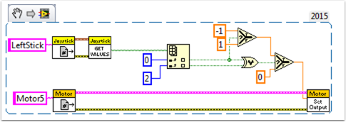
Here I used joystick buttons 0 and 2, but feel free to use whatever buttons you need.
Scenario 2
“I want different joystick buttons move at various speeds.”
This example could be helpful if you need to have one motor do different things based on the buttons you press. For instance, let’s say my joystick has a trigger (button 0) and 4 buttons on top (buttons 1 through 4). In this case, the following buttons should have the following functions:
button 1 - move backward at half speed
button 2 - move forward at half speed
button 3 - move backward at 1/4 speed
button 4 - move forward at 1/4 speed
trigger - full speed ahead! (forward at full speed)
We would then take the boolean array from the “JoystickGetValues.vi” and wire it to a “Boolean Array to Number” node (Numeric Palette-Conversion Palette). This converts the boolean array to a number that we can use. Wire this numeric to a case structure.
Each case corresponds to a binary representation of the values in the array. In this example, each case corresponds to a one-button combination. We added six cases: 0 (all buttons off), 1 (button 0 on), 2 (button 1 on), 4 (button 2 on), 8 (button 3 on), and 16 (button 4 on). Notice we skipped value 3. 3 would correspond to buttons 0 and 1 pressed at the same time. We did not define this in our requirements so we’ll let the default case handle it.
It might be helpful to review the LabVIEW 2014 Case Structure Help document here:
https://zone.ni.com/reference/en-XX/help/371361L-01/glang/case_structure/
There are also 3 Community Tutorials on case structures here:
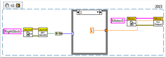
Since our requirements were simple, we only need a single constant in each case. For case 1 (full ahead) we use a 1, for case 2 (half back) we use a -0.5, etc. We can use any constant value between 1 and -1. I left case 0 as the default so if multiple buttons are pressed (any undefined state was reached) the motor will stop. You of course are free to customize these states however you want.
Scenario 3
“I want to control a solenoid with my joystick buttons.”
By now, we are familiar with how the joystick outputs the buttons in an array of booleans. We need to index this array to get the button we are interested in, and wire this boolean to a select node. Since the “Solenoid Set.vi” requires a Enum as an input, the easiest way to get the enum is to right click the “Value” input of the “Solenoid Set.vi” and select “Create Constant”. Duplicate this constant and wire one copy to the True terminal and one to the False terminal of the select node. Then wire the output of the select node to the “Value” input of the solenoid VI.
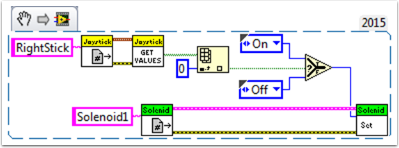
Happy Roboting!
Local and Global Variables in LabVIEW for FRC
This example serves as an introduction to local and global variables, how they are used in the default LabVIEW for FRC® Robot Project, and how you might want to use them in your project.
Local variables and global variables may be used to transfer data between locations within the same VI (local variables) or within different VI’s (global variables), breaking the conventional Data Flow Paradigm for which LabVIEW is famous. Thus, they may be useful when, for whatever reason, you cannot wire the value directly to the node to another.
Note: One possible reason may be that you need to pass data between consecutive loop iterations; Miro_T covered this in this post. It should also be noted that the feedback node in LabVIEW may be used as an equivalent to the shift register, although that may be a topic for another day!
Introduction to Local and Global Variables
Local variables may be used within the same VI. Create a local variable by right-clicking a control or indicator on your Front Panel:
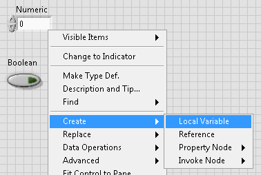
You may create a local variable from the Structures palette on the block diagram as well. When you have multiple local variables in one VI, you can left-click to choose which variable it is:
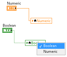
Global variables are created slightly differently. Add one to the block diagram from the Structures palette, and notice that when you double-click it, it opens a separate front panel. This front panel does not have a block diagram, but you add as many entities to the front panel as you wish and save it as a *.vi file:
Note
Be very careful to avoid race conditions when using local and global variables! Essentially, make sure that you are not accidentally writing to the same variable in multiple locations without a way to know to which location it was last written. For a more thorough explanation, see this help document
How They are Used in the Default LabVIEW for FRC Robot Project
Global variables for “Enable Vision” and “Image Size” are written to during each iteration of the Robot Main VI…
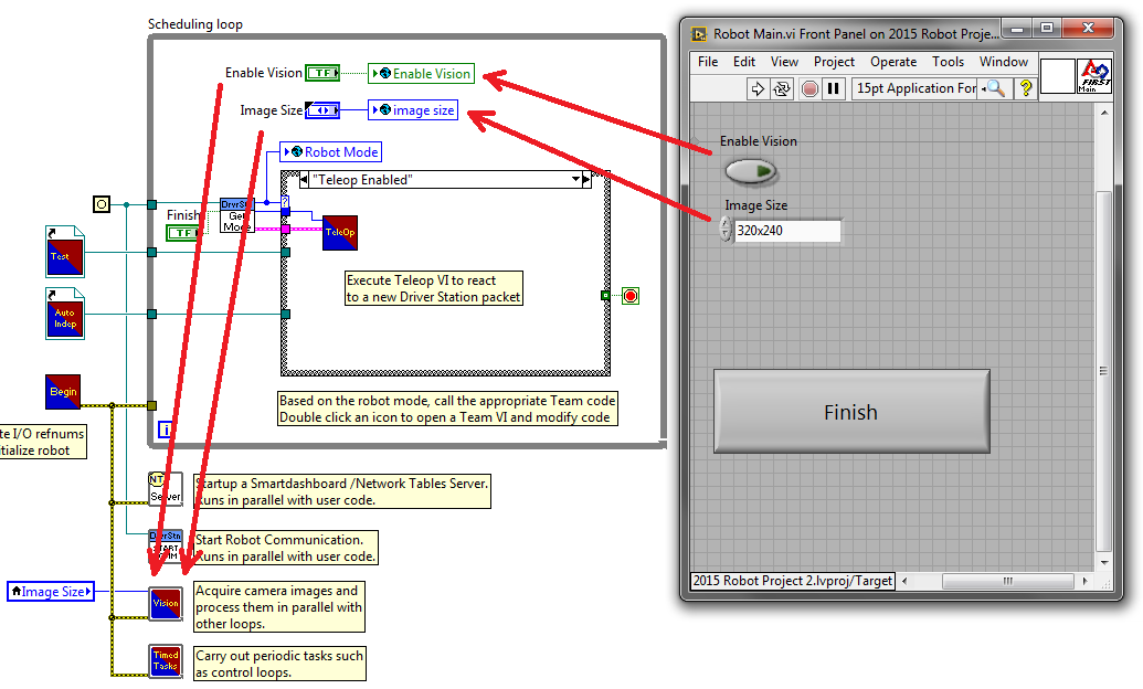
… And then read in each iteration of the Vision Processing VI:
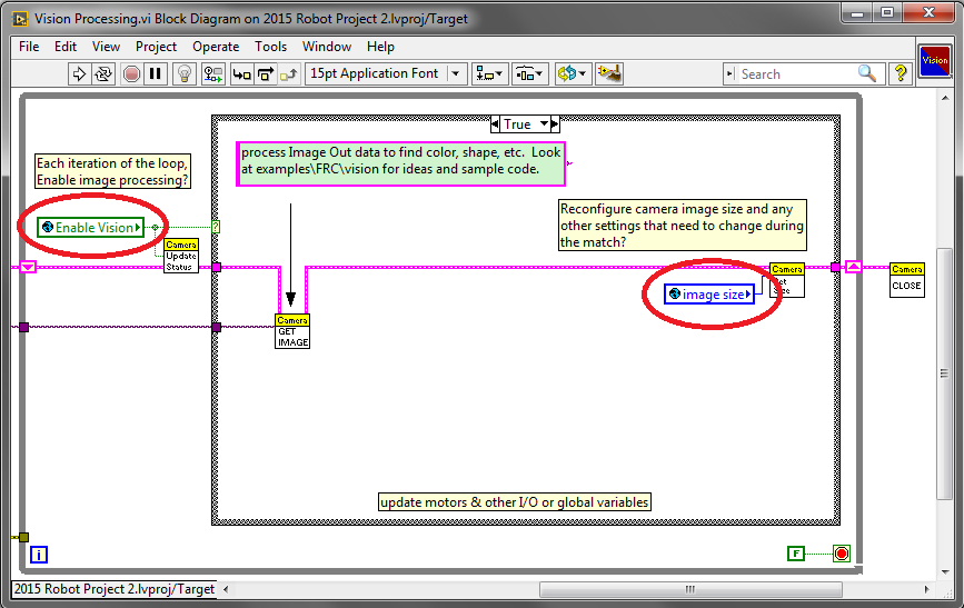
This allows the user, when deploying to Robot Main VI from the LabVIEW Development Environment, to enable/disable vision and change the image size from Robot Main’s Front Panel.
How Can You Use Them in Your Project?
Check out the block diagram for the Periodic Tasks VI. Perhaps there is some value, such as a boolean, that may be written to a global variable in the Teleop VI, and then read from in the Periodic Tasks VI. You can then decide what code or values to use in the Periodic Tasks VI, depending on the boolean global variable:
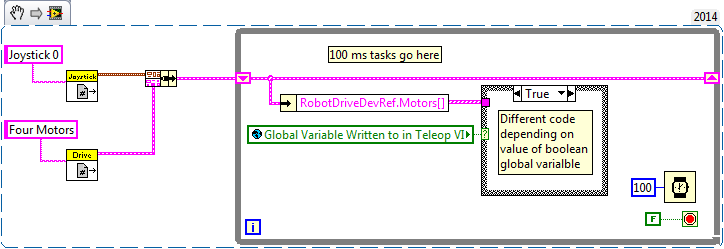
Using the Compressor in LabVIEW
This snippet shows how to set up your roboRIO project to use the Pneumatic Control Module (PCM). The PCM automatically starts and stops the compressor when specific pressures are measured in the tank. In your roboRIO program, you will need to add the following VIs.
For more information, check out the following links:
Pneumatics Step by Step for the roboRIO
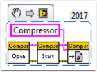
Teleop VI
Place this snippet in the Teleop.vi. This portion is only required if you are using the outputs for other processes.
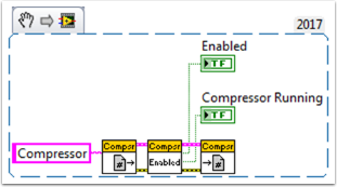
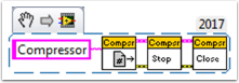
Hardware APIs
This section discusses the control of motors and pneumatics through motor controllers, solenoids and pneumatics, and their interface with Java and C++ WPILib.
Motors APIs
Programming your motors are absolutely essential to a moving robot! This section showcases some helpful classes and examples for getting your robot up and moving!
Using Motor Controllers in Code
Motor controllers come in two main flavors: CAN and PWM. A CAN controller can send more detailed status information back to the roboRIO, whereas a PWM controller can only be set to a value. For information on using these motors with the WPI drivetrain classes, see Using the WPILib Classes to Drive your Robot.
Using PWM Motor Controllers
PWM motor controllers can be controlled in the same way as a CAN motor controller. For a more detailed background on how they work, see PWM Motor Controllers in Depth. To use a PWM motor controller, simply use the appropriate motor controller class provided by WPI and supply it the port the motor controller(s) are plugged into on the roboRIO. All approved motor controllers have WPI classes provided for them.
Spark spark = new Spark(0); // 0 is the RIO PWM port this is connected to

spark.set(-0.75); // the % output of the motor, between -1 and 1

VictorSP victor = new VictorSP(0); // 0 is the RIO PWM port this is connected to

victor.set(0.6); // the % output of the motor, between -1 and 1
frc::Spark spark{0}; // 0 is the RIO PWM port this is connected to

spark.Set(-0.75); // the % output of the motor, between -1 and 1

frc::VictorSP victor{0}; // 0 is the RIO PWM port this is connected to

victor.Set(0.6); // the % output of the motor, between -1 and 1
CAN Motor Controllers
A handful of CAN motor controllers are available through vendors such as CTR Electronics and REV Robotics.
SPARK MAX
For information regarding the SPARK MAX CAN Motor Controller, which can be used in either CAN or PWM mode, please refer to the SPARK MAX software resources and example code.
PWM Motor Controllers in Depth
Hint
WPILib has extensive support for motor control. There are a number of classes that represent different types of motor controllers and servos. There are currently two classes of motor controllers, PWM based motor controllers and CAN based motor controllers. WPILib also contains composite classes (like DifferentialDrive) which allow you to control multiple motors with a single object. This article will cover the details of PWM motor controllers; CAN controllers and composite classes will be covered in separate articles.
PWM Controllers, brief theory of operation
The acronym PWM stands for Pulse Width Modulation. For motor controllers, PWM can refer to both the input signal and the method the controller uses to control motor speed. To control the speed of the motor the controller must vary the perceived input voltage of the motor. To do this the controller switches the full input voltage on and off very quickly, varying the amount of time it is on based on the control signal. Because of the mechanical and electrical time constants of the types of motors used in FRC® this rapid switching produces an effect equivalent to that of applying a fixed lower voltage (50% switching produces the same effect as applying ~6V).
The PWM signal the controllers use for an input is a little bit different. Even at the bounds of the signal range (max forward or max reverse) the signal never approaches a duty cycle of 0% or 100%. Instead the controllers use a signal with a period of either 5ms or 10ms and a midpoint pulse width of 1.5ms. Many of the controllers use the typical hobby RC controller timing of 1ms to 2ms.
Raw vs Scaled output values
In general, all of the motor controller classes in WPILib take a scaled -1.0 to 1.0 value as the output to an actuator. The PWM module in the FPGA on the roboRIO is capable of generating PWM signals with periods of 5, 10, or 20ms and can vary the pulse width in 2000 steps of ~.001ms each around the midpoint (1000 steps in each direction around the midpoint). The raw values sent to this module are in this 0-2000 range with 0 being a special case which holds the signal low (disabled). The class for each motor controller contains information about what the typical bound values (min, max and each side of the deadband) are as well as the typical midpoint. WPILib can then use these values to map the scaled value into the proper range for the motor controller. This allows for the code to switch seamlessly between different types of controllers and abstracts out the details of the specific signaling.
Calibrating Motor Controllers
So if WPILib handles all this scaling, why would you ever need to calibrate your motor controller? The values WPILib uses for scaling are approximate based on measurement of a number of samples of each controller type. Due to a variety of factors, the timing of an individual motor controller may vary slightly. In order to definitively eliminate “humming” (midpoint signal interpreted as slight movement in one direction) and drive the controller all the way to each extreme, calibrating the controllers is still recommended. In general, the calibration procedure for each controller involves putting the controller into calibration mode then driving the input signal to each extreme, then back to the midpoint. For examples on how to use these motor controllers in your code, see Using Motor Controllers in Code/Using PWM Motor Controllers
Using the WPILib Classes to Drive your Robot
WPILib includes many classes to help make your robot get driving faster.
Standard drivetrains
Differential Drive Robots
These drive bases typically have two or more in-line traction or omni wheels per side (e.g., 6WD or 8WD) and may also be known as “skid-steer”, “tank drive”, or “West Coast Drive”. The Kit of Parts drivetrain is an example of a differential drive. These drivetrains are capable of driving forward/backward and can turn by driving the two sides in opposite directions causing the wheels to skid sideways. These drivetrains are not capable of sideways translational movement.
Mecanum Drive
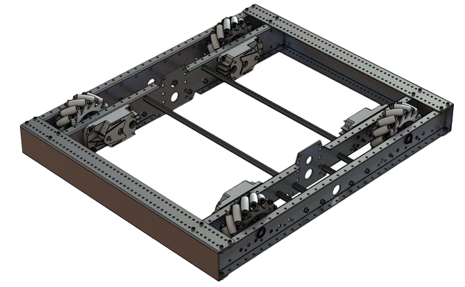
Mecanum drive is a method of driving using specially designed wheels that allow the robot to drive in any direction without changing the orientation of the robot. A robot with a conventional drivetrain (all wheels pointing in the same direction) must turn in the direction it needs to drive. A mecanum robot can move in any direction without first turning and is called a holonomic drive. The wheels (shown on this robot) have rollers that cause the forces from driving to be applied at a 45 degree angle rather than straight forward as in the case of a conventional drive.
When viewed from the top, the rollers on a mecanum drivetrain should form an ‘X’ pattern. This results in the force vectors (when driving the wheel forward) on the front two wheels pointing forward and inward and the rear two wheels pointing forward and outward. By spinning the wheels in different directions, various components of the force vectors cancel out, resulting in the desired robot movement. A quick chart of different movements has been provided below, drawing out the force vectors for each of these motions may help in understanding how these drivetrains work. By varying the speeds of the wheels in addition to the direction, movements can be combined resulting in translation in any direction and rotation, simultaneously.
Drive Class Conventions
Motor Inversion
As of 2022, the right side of the drivetrain is no longer inverted by default. It is the responsibility of the user to manage proper inversions for their drivetrain. Users can invert motors by calling setInverted()/SetInverted() on their motor objects.
PWMSparkMax m_motorRight = new PWMSparkMax(0);

@Override
public void robotInit() {
   m_motorRight.setInverted(true);
}
frc::PWMSparkMax m_motorLeft{0};

public:
 void RobotInit() override {
   m_motorRight.SetInverted(true);
 }
Squaring Inputs
When driving robots, it is often desirable to manipulate the joystick inputs such that the robot has finer control at low speeds while still using the full output range. One way to accomplish this is by squaring the joystick input, then reapplying the sign. By default the Differential Drive class will square the inputs. If this is not desired (e.g. if passing values in from a PIDController), use one of the drive methods with the squaredInputs parameter and set it to false.
Input Deadband
By default, the Differential Drive class applies an input deadband of 0.02. This means that input values with a magnitude below 0.02 (after any squaring as described above) will be set to 0. In most cases these small inputs result from imperfect joystick centering and are not sufficient to cause drivetrain movement, the deadband helps reduce unnecessary motor heating that may result from applying these small values to the drivetrain. To change the deadband, use the setDeadband() method.
Maximum Output
Sometimes drivers feel that their drivetrain is driving too fast and want to limit the output. This can be accomplished with the setMaxOutput() method. This maximum output is multiplied by result of the previous drive functions like deadband and squared inputs.
Motor Safety
Motor Safety is a mechanism in WPILib that takes the concept of a watchdog and breaks it out into one watchdog (Motor Safety timer) for each individual actuator. Note that this protection mechanism is in addition to the System Watchdog which is controlled by the Network Communications code and the FPGA and will disable all actuator outputs if it does not receive a valid data packet for 125ms.
The purpose of the Motor Safety mechanism is the same as the purpose of a watchdog timer, to disable mechanisms which may cause harm to themselves, people or property if the code locks up and does not properly update the actuator output. Motor Safety breaks this concept out on a per actuator basis so that you can appropriately determine where it is necessary and where it is not. Examples of mechanisms that should have motor safety enabled are systems like drive trains and arms. If these systems get latched on a particular value they could cause damage to their environment or themselves. An example of a mechanism that may not need motor safety is a spinning flywheel for a shooter. If this mechanism gets latched on a particular value it will simply continue spinning until the robot is disabled. By default Motor Safety is enabled for DifferentialDrive, KilloughDrive, and MecanumDrive objects and disabled for all other motor controllers and servos.
The Motor Safety feature operates by maintaining a timer that tracks how long it has been since the feed() method has been called for that actuator. Code in the Driver Station class initiates a comparison of these timers to the timeout values for any actuator with safety enabled every 5 received packets (100ms nominal). The set() methods of each motor controller class and the set() and setAngle() methods of the servo class call feed() to indicate that the output of the actuator has been updated.
The Motor Safety interface of motor controllers can be interacted with by the user using the following methods:
exampleJaguar.setSafetyEnabled(true);
exampleJaguar.setSafetyEnabled(false);
exampleJaguar.setExpiration(.1);
exampleJaguar.feed()
exampleJaguar->SetSafetyEnabled(true);
exampleJaguar->SetSafetyEnabled(false);
exampleJaguar->SetExpiration(.1);
exampleJaguar->Feed();
By default all Drive objects enable Motor Safety. Depending on the mechanism and the structure of your program, you may wish to configure the timeout length of the motor safety (in seconds). The timeout length is configured on a per actuator basis and is not a global setting. The default (and minimum useful) value is 100ms.
Axis Conventions
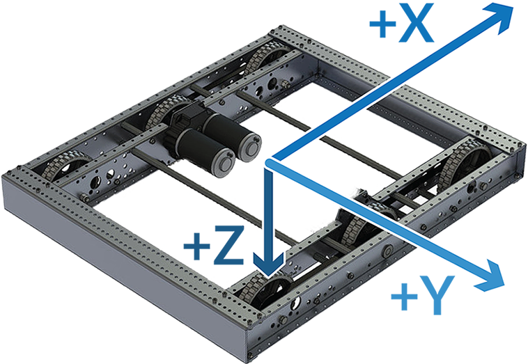
The drive classes use the NED axes convention (North-East-Down as external reference in the world frame). The positive X axis points ahead, the positive Y axis points right, and the positive Z axis points down. The rest of the library, and math in general, uses NWU axes convention (North-West-Up). We use NED here because joysticks use NED, and they use NED because the aviation industry does.
Joysticks follow NED convention, but it’s important to note that axes values are rotations around the respective axes, not translations. When viewed with each axis pointing toward you, CCW is a positive value and CW is a negative value. Pushing forward on the joystick is a CW rotation around the Y axis, so you get a negative value. Pushing to the right is a CCW rotation around the X axis, so you get a positive value.
Using the DifferentialDrive class to control Differential Drive robots
Note
WPILib provides separate Robot Drive classes for the most common drive train configurations (differential, mecanum, and Killough). The DifferentialDrive class handles the differential drivetrain configuration. These drive bases typically have two or more in-line traction or omni wheels per side (e.g., 6WD or 8WD) and may also be known as “skid-steer”, “tank drive”, or “West Coast Drive” (WCD). The Kit of Parts drivetrain is an example of a differential drive. There are methods to control the drive with 3 different styles (“Tank”, “Arcade”, or “Curvature”), explained in the article below.
DifferentialDrive is a method provided for the control of “skid-steer” or “West Coast” drivetrains, such as the Kit of Parts chassis. Instantiating a DifferentialDrive is as simple as so:
public class Robot {
    Spark m_left = new Spark(1);
    Spark m_right = new Spark(2);
    DifferentialDrive m_drive = new DifferentialDrive(m_left, m_right);

    public void robotInit() {
        m_left.setInverted(true); // if you want to invert motor outputs, you must do so here
    }
class Robot {
    private:
        frc::Spark m_left{1};
        frc::Spark m_right{2};
        frc::DifferentialDrive m_drive{m_left, m_right};
void Robot::RobotInit() {
    m_left.SetInverted(true); // if you want to invert motor outputs, you must do so here
}
Multi-Motor DifferentialDrive with MotorControllerGroups
Many FRC® drivetrains have more than 1 motor on each side. In order to use these with DifferentialDrive, the motors on each side have to be collected into a single MotorController, using the MotorControllerGroup class. The examples below show a 4 motor (2 per side) drivetrain. To extend to more motors, simply create the additional controllers and pass them all into the MotorController group constructor (it takes an arbitrary number of inputs).
public class Robot {
    Spark m_frontLeft = new Spark(1);
    Spark m_rearLeft = new Spark(2);
    MotorControllerGroup m_left = new MotorControllerGroup(m_frontLeft, m_rearLeft);

    Spark m_frontRight = new Spark(3);
    Spark m_rearRight = new Spark(4);
    MotorControllerGroup m_right = new MotorControllerGroup(m_frontRight, m_rearRight);
    DifferentialDrive m_drive = new DifferentialDrive(m_left, m_right);

    public void robotInit() {
        m_left.setInverted(true); // if you want to invert the entire side you can do so here
    }
class Robot {
    public:
        frc::Spark m_frontLeft{1};
        frc::Spark m_rearLeft{2};
        frc::MotorControllerGroup m_left{m_frontLeft, m_rearLeft};

        frc::Spark m_frontRight{3};
        frc::Spark m_rearRight{4};
        frc::MotorControllerGroup m_right{m_frontRight, m_rearRight};

        frc::DifferentialDrive m_drive{m_left, m_right};
void Robot::RobotInit() {
    m_left.SetInverted(true); // if you want to invert the entire side you can do so here
}
Drive Modes
Note
The DifferentialDrive class contains three different default modes of driving your robot’s motors.
Tank Drive, which controls the left and right side independently
Arcade Drive, which controls a forward and turn speed
Curvature Drive, a subset of Arcade Drive, which makes your robot handle like a car with constant-curvature turns.
The DifferentialDrive class contains three default methods for controlling skid-steer or WCD robots. Note that you can create your own methods of controlling the robot’s driving and have them call tankDrive() with the derived inputs for left and right motors.
The Tank Drive mode is used to control each side of the drivetrain independently (usually with an individual joystick axis controlling each). This example shows how to use the Y-axis of two separate joysticks to run the drivetrain in Tank mode. Construction of the objects has been omitted, for above for drivetrain construction and here for Joystick construction.
The Arcade Drive mode is used to control the drivetrain using speed/throttle and rotation rate. This is typically used either with two axes from a single joystick, or split across joysticks (often on a single gamepad) with the throttle coming from one stick and the rotation from another. This example shows how to use a single joystick with the Arcade mode. Construction of the objects has been omitted, for above for drivetrain construction and here for Joystick construction.
Like Arcade Drive, the Curvature Drive mode is used to control the drivetrain using speed/throttle and rotation rate. The difference is that the rotation control input controls the radius of curvature instead of rate of heading change, much like the steering wheel of a car. This mode also supports turning in place, which is enabled when the third boolean parameter is true.
public void teleopPeriodic() {
    // Tank drive with a given left and right rates
    myDrive.tankDrive(-leftStick.getY(), -rightStick.getY());

    // Arcade drive with a given forward and turn rate
    myDrive.arcadeDrive(-driveStick.getY(), driveStick.getX());

    // Curvature drive with a given forward and turn rate, as well as a button for turning in-place.
    myDrive.curvatureDrive(-driveStick.getY(), driveStick.getX(), driveStick.getButton(1));
}
void TeleopPeriodic() override {
    // Tank drive with a given left and right rates
    myDrive.TankDrive(-leftStick.GetY(), -rightStick.GetY());

    // Arcade drive with a given forward and turn rate
    myDrive.ArcadeDrive(-driveStick.GetY(), driveStick.GetX());

    // Curvature drive with a given forward and turn rate, as well as a quick-turn button
    myDrive.CurvatureDrive(-driveStick.GetY(), driveStick.GetX(), driveStick.GetButton(1));
}
Using the MecanumDrive class to control Mecanum Drive robots
MecanumDrive is a method provided for the control of holonomic drivetrains with Mecanum wheels, such as the Kit of Parts chassis with the mecanum drive upgrade kit, as shown above. Instantiating a MecanumDrive is as simple as so:
24  @Override
25  public void robotInit() {
26    PWMSparkMax frontLeft = new PWMSparkMax(kFrontLeftChannel);
27    PWMSparkMax rearLeft = new PWMSparkMax(kRearLeftChannel);
28    PWMSparkMax frontRight = new PWMSparkMax(kFrontRightChannel);
29    PWMSparkMax rearRight = new PWMSparkMax(kRearRightChannel);
30
31    // Invert the right side motors.
32    // You may need to change or remove this to match your robot.
33    frontRight.setInverted(true);
34    rearRight.setInverted(true);
35
36    m_robotDrive = new MecanumDrive(frontLeft, rearLeft, frontRight, rearRight);
37
38    m_stick = new Joystick(kJoystickChannel);
39  }
30 private:
31  static constexpr int kFrontLeftChannel = 0;
32  static constexpr int kRearLeftChannel = 1;
33  static constexpr int kFrontRightChannel = 2;
34  static constexpr int kRearRightChannel = 3;
35
36  static constexpr int kJoystickChannel = 0;
37
38  frc::PWMSparkMax m_frontLeft{kFrontLeftChannel};
39  frc::PWMSparkMax m_rearLeft{kRearLeftChannel};
40  frc::PWMSparkMax m_frontRight{kFrontRightChannel};
41  frc::PWMSparkMax m_rearRight{kRearRightChannel};
42  frc::MecanumDrive m_robotDrive{m_frontLeft, m_rearLeft, m_frontRight,
43                                 m_rearRight};
Mecanum Drive Modes
Note
The drive axis conventions are different from common joystick axis conventions. See the Axis Conventions above for more information.
The MecanumDrive class contains two different default modes of driving your robot’s motors.
driveCartesian: Angles are measured clockwise from the positive X axis. The robot’s speed is independent from its angle or rotation rate.
drivePolar: Angles are measured counter-clockwise from straight ahead. The speed at which the robot drives (translation) is independent from its angle or rotation rate.
public void teleopPeriodic() {
    m_robotDrive.driveCartesian(m_stick.getX(), -m_stick.getY(), m_stick.getZ());
    m_robotDrive.drivePolar(m_stick.getX(), -m_stick.getY(), m_stick.getZ());
}
void TeleopPeriodic() override {
    m_robotDrive.driveCartesian(m_stick.GetX(), -m_stick.GetY(), m_stick.GetZ());
    m_robotDrive.drivePolar(m_stick.GetX(), -m_stick.GetY(), m_stick.GetZ());
}
Field-Oriented Driving
A 4th parameter can be supplied to the driveCartesian(double ySpeed, double xSpeed, double zRotation, double gyroAngle) method, the angle returned from a Gyro sensor. This will adjust the rotation value supplied. This is particularly useful with mecanum drive since, for the purposes of steering, the robot really has no front, back or sides. It can go in any direction. Adding the angle in degrees from a gyro object will cause the robot to move away from the drivers when the joystick is pushed forwards, and towards the drivers when it is pulled towards them, regardless of what direction the robot is facing.
The use of field-oriented driving makes often makes the robot much easier to drive, especially compared to a “robot-oriented” drive system where the controls are reversed when the robot is facing the drivers.
Just remember to get the gyro angle each time driveCartesian() is called.
Note
Many teams also like to ramp the joysticks inputs over time to promote a smooth acceleration and reduce jerk. This can be accomplished with a Slew Rate Limiter.
Repeatable Low Power Movement - Controlling Servos with WPILib
Servo motors are a type of motor which integrates positional feedback into the motor in order to allow a single motor to perform repeatable, controllable movement, taking position as the input signal. WPILib provides the capability to control servos which match the common hobby input specification (Pulse Width Modulation (PWM) signal, 0.6 ms - 2.4 ms pulse width)
Constructing a Servo object
Servo exampleServo = new Servo(1);
frc::Servo exampleServo {1};
A servo object is constructed by passing a channel.
Setting Servo Values
exampleServo.set(.5);
exampleServo.setAngle(75);
exampleServo.Set(.5);
exampleServo.SetAngle(75);
There are two methods of setting servo values in WPILib:
Scaled Value - Sets the servo position using a scaled 0 to 1.0 value. 0 corresponds to one extreme of the servo and 1.0 corresponds to the other
Angle - Set the servo position by specifying the angle, in degrees from 0 to 180. This method will work for servos with the same range as the Hitec HS-322HD servo . Any values passed to this method outside the specified range will be coerced to the boundary.
Pneumatics APIs
Operating pneumatic cylinders
Using the FRC Control System to control Pneumatics
There are two options for operating solenoids to control pneumatic cylinders, the CTRE Pneumatics Control Module and the REV Robotics Pneumatics Hub.
The CTRE Pneumatics Control Module (PCM) is a CAN-based device that provides control over the compressor and up to 8 solenoids per module.
The REV Pneumatic Hub (PH) is a CAN-based device that provides control over the compressor and up to 16 solenoids per module.
These devices are integrated into WPILib through a series of classes that make them simple to use. The closed loop control of the Compressor and Pressure switch is handled by the PCM hardware and the Solenoids are handled by the Solenoid class that controls the solenoid channels.
These modules are responsible for regulating the robot’s pressure using a pressure switch and a compressor and switching solenoids on and off. They communicate with the roboRIO over CAN. For more information, see Hardware Component Overview
Module Numbers
CAN Devices are identified by their Node ID. The default Node ID for PCMs is 0. The default Node ID for PHs is 1. If using a single module on the bus it is recommended to leave it at the default Node ID. Additional modules can be used where the modules corresponding solenoids are differentiated by the module number in the constructors of the Solenoid and Compressor classes.
Generating and Storing Pressure
Pressure is created using a pneumatic compressor and stored in pneumatic tanks. The compressor doesn’t necessarily have to be on the robot, but must be powered by the robot’s pneumatics module. The “Closed Loop” mode on the Compressor is enabled by default, and it is not recommended that teams change this setting. When closed loop control is enabled the pneumatic module will automatically turn the compressor on when the digital pressure switch is closed (below the pressure threshold) and turn it off when the pressure switch is open (~120PSI). When closed loop control is disabled the compressor will not be turned on. Using the Compressor (Java / C++) class, users can query the status of the compressor. The state (currently on or off), pressure switch state, and compressor current can all be queried from the Compressor object.
Note
The Compressor object is only needed if you want the ability to turn off the compressor, change the pressure sensor (PH only), or query compressor status.
Compressor pcmCompressor = new Compressor(0, PneumaticsModuleType.CTREPCM);
Compressor phCompressor = new Compressor(1, PneumaticsModuleType.REVPH);

pcmCompressor.enableDigital();
pcmCompressor.disable();

boolean enabled = pcmCompressor.enabled();
boolean pressureSwitch = pcmCompressor.getPressureSwitchValue();
double current = pcmCompressor.getCompressorCurrent();
frc::Compressor pcmCompressor{0, frc::PneumaticsModuleType::CTREPCM};
frc::Compressor phCompressor{1, frc::PneumaticsModuleType::REVPH};

pcmCompressor.EnableDigital();
pcmCompressor.Disable();

bool enabled = pcmCompressor.Enabled();
bool pressureSwitch = pcmCompressor.GetPressureSwitchValue();
double current = pcmCompressor.GetCompressorCurrent();
The Pneumatic Hub also has methods for enabling compressor control using the REV Analog Pressure Sensor (enableAnalog method).
Solenoid control
FRC teams use solenoids to perform a variety of tasks, from shifting gearboxes to operating robot mechanisms. A solenoid is a valve used to electronically switch a pressurized air line “on” or “off”. For more information on solenoids, see this wikipedia article. Solenoids are controlled by a robot’s Pneumatics Control Module, or Pneumatic Hub, which is in turn connected to the robot’s roboRIO via CAN. The easiest way to see a solenoid’s state is via the LEDs on the PCM or PH (which indicates if the valve is “on” or not). When un-powered, solenoids can be manually actuated with the small button on the solenoid.
Single acting solenoids apply or vent pressure from a single output port. They are typically used either when an external force will provide the return action of the cylinder (spring, gravity, separate mechanism) or in pairs to act as a double solenoid. A double solenoid switches air flow between two output ports (many also have a center position where neither output is vented or connected to the input). Double solenoid valves are commonly used when you wish to control both the extend and retract actions of a cylinder using air pressure. Double solenoid valves have two electrical inputs which connect back to two separate channels on the solenoid breakout.
Single Solenoids in WPILib
Single solenoids in WPILib are controlled using the Solenoid class (Java / C++). To construct a Solenoid object, simply pass the desired port number (assumes default CAN ID) and pneumatics module type or CAN ID, pneumatics module type, and port number to the constructor. To set the value of the solenoid call set(true) to enable or set(false) to disable the solenoid output.
Solenoid exampleSolenoidPCM = new Solenoid(PneumaticsModuleType.CTREPCM, 1);
Solenoid exampleSolenoidPH = new Solenoid(PneumaticsModuleType.REVPH, 1);

exampleSolenoidPCM.set(true);
exampleSolenoidPCM.set(false);
frc::Solenoid exampleSolenoidPCM{frc::PneumaticsModuleType::CTREPCM, 1};
frc::Solenoid exampleSolenoidPH{frc::PneumaticsModuleType::REVPH, 1};

exampleSolenoidPCM.Set(true);
exampleSolenoidPCM.Set(false);
Double Solenoids in WPILib
Double solenoids are controlled by the DoubleSolenoid class in WPILib (Java / C++. These are constructed similarly to the single solenoid but there are now two port numbers to pass to the constructor, a forward channel (first) and a reverse channel (second). The state of the valve can then be set to kOff (neither output activated), kForward (forward channel enabled) or kReverse (reverse channel enabled). Additionally, the CAN ID can be passed to the DoubleSolenoid if teams have a non-standard CAN ID.
// Using "import static an.enum.or.constants.inner.class.*;" helps reduce verbosity
// this replaces "DoubleSolenoid.Value.kForward" with just kForward
// further reading is available at https://www.geeksforgeeks.org/static-import-java/
import static edu.wpi.first.wpilibj.DoubleSolenoid.Value.*;

DoubleSolenoid exampleDoublePCM = new DoubleSolenoid(PneumaticsModuleType.CTREPCM, 1, 2);
DoubleSolenoid exampleDoublePH = new DoubleSolenoid(9, PneumaticsModuleType.REVPH, 4, 5);


exampleDoublePCM.set(kOff);
exampleDoublePCM.set(kForward);
exampleDoublePCM.set(kReverse);
frc::DoubleSolenoid exampleDoublePCM{frc::PneumaticsModuleType::CTREPCM, 1, 2};
frc::DoubleSolenoid exampleDoublePH{9, frc::PneumaticsModuleType::REVPH, 4, 5};

exampleDoublePCM.Set(frc::DoubleSolenoid::Value::kOff);
exampleDoublePCM.Set(frc::DoubleSolenoid::Value::kForward);
exampleDoublePCM.Set(frc::DoubleSolenoid::Value::kReverse);
Toggling Solenoids
Solenoids can be switched from one output to the other (known as toggling) by using the .toggle() method.
Note
Since a DoubleSolenoid defaults to off, you will have to set it before it can be toggled.
Solenoid exampleSingle = new Solenoid(PneumaticsModuleType.CTREPCM, 0);
DoubleSolenoid exampleDouble = new DoubleSolenoid(PneumaticsModuleType.CTREPCM, 1, 2);

// Initialize the DoubleSolenoid so it knows where to start.  Not required for single solenoids.
exampleDouble.set(kReverse);

if (m_controller.getYButtonPressed()) {
   exampleSingle.toggle();
   exampleDouble.toggle();
}
frc::Solenoid exampleSingle{frc::PneumaticsModuleType::CTREPCM, 0};
frc::DoubleSolenoid exampleDouble{frc::PneumaticsModuleType::CTREPCM, 1, 2};

// Initialize the DoubleSolenoid so it knows where to start.  Not required for single solenoids.
exampleDouble.Set(frc::DoubleSolenoid::Value::kReverse);

if (m_controller.GetYButtonPressed()) {
   exampleSingle.Toggle();
   exampleDouble.Toggle();
}
Pressure Transducers
A pressure transducer is a sensor where analog voltage is proportial to the measured pressure.
Pneumatic Hub
The Pneumatic Hub has analog inputs that may be used to read a pressure transducer using the Compressor class.
Compressor phCompressor = new Compressor(1, PneumaticsModuleType.REVPH);

double current = phCompressor.getPressure();
#include <units/pressure.h>

frc::Compressor phCompressor{1, frc::PneumaticsModuleType::REVPH};

units::pounds_per_square_inch_t current = phCompressor.GetPressure();
roboRIO
A pressure transducer can be connected to the Analog Input ports on the roboRIO, and can be read by the AnalogInput or AnalogPotentiometer classes in WPILib.
import edu.wpi.first.wpilibj.AnalogInput;
import edu.wpi.first.wpilibj.AnalogPotentiometer;

// product-specific voltage->pressure conversion, see product manual
// in this case, 250(V/5)-25
// the scale parameter in the AnalogPotentiometer constructor is scaled from 1 instead of 5,
// so if r is the raw AnalogPotentiometer output, the pressure is 250r-25
double scale = 250, offset = -25;
AnalogPotentiometer pressureTransducer = new AnalogPotentiometer(/* the AnalogIn port*/ 2, scale, offset);

// scaled values in psi units
double psi = pressureTransducer.get();
// product-specific voltage->pressure conversion, see product manual
// in this case, 250(V/5)-25
// the scale parameter in the AnalogPotentiometer constructor is scaled from 1 instead of 5,
// so if r is the raw AnalogPotentiometer output, the pressure is 250r-25
double scale = 250, offset = -25;
frc::AnalogPotentiometer pressureTransducer{/* the AnalogIn port*/ 2, scale, offset};

// scaled values in psi units
double psi = pressureTransducer.Get();
Sensors
Sensors are an integral way of having your robot hardware and software communicate with each other. This section highlights interfacing with those sensors at a software level.
Sensor Overview - Software
Note
This section covers using sensors in software. For a guide to sensor hardware, see Sensor Overview - Hardware.
Note
While cameras may definitely be considered “sensors”, vision processing is a sufficiently-complicated subject that it is covered in its own section, rather than here.
In order to be effective, it is often vital for robots to be able to gather information about their surroundings. Devices that provide feedback to the robot on the state of its environment are called “sensors.” WPILib innately supports a large variety of sensors through classes included in the library. This section will provide a guide to both using common sensor types through WPILib, as well as writing code for sensors without official support.
What sensors does WPILIB support?
The roboRIO includes a FPGA which allows accurate real-time measuring of a variety of sensor input. WPILib, in turn, provides a number of classes for accessing this functionality.
WPILib provides native support for:
Additionally, WPILib includes lower-level classes for interfacing directly with the FPGA’s digital and analog inputs and outputs.
Accelerometers - Software
Note
This section covers accelerometers in software. For a hardware guide to accelerometers, see Accelerometers - Hardware.
An accelerometer is a device that measures acceleration.
Accelerometers generally come in two types: single-axis and 3-axis. A single-axis accelerometer measures acceleration along one spatial dimension; a 3-axis accelerometer measures acceleration along all three spatial dimensions at once.
WPILib supports single-axis accelerometers through the AnalogAccelerometer class.
Three-axis accelerometers often require more complicated communications protocols (such as SPI or I2C) in order to send multi-dimensional data. WPILib has native support for the following 3-axis accelerometers:
AnalogAccelerometer
The AnalogAccelerometer class (Java, C++) allows users to read values from a single-axis accelerometer that is connected to one of the roboRIO’s analog inputs.
// Creates an analog accelerometer on analog input 0
AnalogAccelerometer accelerometer = new AnalogAccelerometer(0);

// Sets the sensitivity of the accelerometer to 1 volt per G
accelerometer.setSensitivity(1);

// Sets the zero voltage of the accelerometer to 3 volts
accelerometer.setZero(3);

// Gets the current acceleration
double accel = accelerometer.getAcceleration();
// Creates an analog accelerometer on analog input 0
frc::AnalogAccelerometer accelerometer{0};

// Sets the sensitivity of the accelerometer to 1 volt per G
accelerometer.SetSensitivity(1);

// Sets the zero voltage of the accelerometer to 3 volts
accelerometer.SetZero(3);

// Gets the current acceleration
double accel = accelerometer.GetAcceleration();
If users have a 3-axis analog accelerometer, they can use three instances of this class, one for each axis.
The Accelerometer interface
All 3-axis accelerometers in WPILib implement the Accelerometer interface (Java, C++). This interface defines functionality and settings common to all supported 3-axis accelerometers.
The Accelerometer interface contains getters for the acceleration along each cardinal direction (x, y, and z), as well as a setter for the range of accelerations the accelerometer will measure.
Warning
Not all accelerometers are capable of measuring all ranges.
// Sets the accelerometer to measure between -8 and 8 G's
accelerometer.setRange(Accelerometer.Range.k8G);
// Sets the accelerometer to measure between -8 and 8 G's
accelerometer.SetRange(Accelerometer::Range::kRange_8G);
ADXL345_I2C
The ADXL345_I2C class (Java, C++) provides support for the ADXL345 accelerometer over the I2C communications bus.
// Creates an ADXL345 accelerometer object on the MXP I2C port
// with a measurement range from -8 to 8 G's
Accelerometer accelerometer = new ADXL345_I2C(I2C.Port.kMXP, Accelerometer.Range.k8G);
// Creates an ADXL345 accelerometer object on the MXP I2C port
// with a measurement range from -8 to 8 G's
frc::ADXL345_I2C accelerometer{I2C::Port::kMXP, Accelerometer::Range::kRange_8G};
ADXL345_SPI
The ADXL345_SPI class (Java, C++) provides support for the ADXL345 accelerometer over the SPI communications bus.
// Creates an ADXL345 accelerometer object on the MXP SPI port
// with a measurement range from -8 to 8 G's
Accelerometer accelerometer = new ADXL345_SPI(SPI.Port.kMXP, Accelerometer.Range.k8G);
// Creates an ADXL345 accelerometer object on the MXP SPI port
// with a measurement range from -8 to 8 G's
frc::ADXL345_SPI accelerometer{SPI::Port::kMXP, Accelerometer::Range::kRange_8G};
ADXL362
The ADXL362 class (Java, C++) provides support for the ADXL362 accelerometer over the SPI communications bus.
// Creates an ADXL362 accelerometer object on the MXP SPI port
// with a measurement range from -8 to 8 G's
Accelerometer accelerometer = new ADXL362(SPI.Port.kMXP, Accelerometer.Range.k8G);
// Creates an ADXL362 accelerometer object on the MXP SPI port
// with a measurement range from -8 to 8 G's
frc::ADXL362 accelerometer{SPI::Port::kMXP, Accelerometer::Range::kRange_8G};
BuiltInAccelerometer
The BuiltInAccelerometer class (Java, C++) provides access to the roboRIO’s own built-in accelerometer:
// Creates an object for the built-in accelerometer
// Range defaults to +- 8 G's
Accelerometer accelerometer = new BuiltInAccelerometer();
// Creates an object for the built-in accelerometer
// Range defaults to +- 8 G's
frc::BuiltInAccelerometer accelerometer{};
Third-party accelerometers
While WPILib provides native support for a number of accelerometers that are available in the kit of parts or through FIRST Choice, there are a few popular AHRS (Attitude and Heading Reference System) devices commonly used in FRC that include accelerometers. These are generally controlled through vendor libraries, though if they have a simple analog output they can be used with the AnalogAccelerometer class.
Using accelerometers in code
Note
Accelerometers, as their name suggests, measure acceleration. Precise accelerometers can be used to determine position through double-integration (since acceleration is the second derivative of position), much in the way that gyroscopes are used to determine heading. However, the accelerometers available for use in FRC are not nearly high-enough quality to be used this way.
It is recommended to use accelerometers in FRC® for any application which needs a rough measurement of the current acceleration. This can include detecting collisions with other robots or field elements, so that vulnerable mechanisms can be automatically retracted. They may also be used to determine when the robot is passing over rough terrain for an autonomous routine (such as traversing the defenses in FIRST Stronghold).
For detecting collisions, it is often more robust to measure the jerk than the acceleration. The jerk is the derivative (or rate of change) of acceleration, and indicates how rapidly the forces on the robot are changing - the sudden impulse from a collision causes a sharp spike in the jerk. Jerk can be determined by simply taking the difference of subsequent acceleration measurements, and dividing by the time between them:
double prevXAccel = 0;
double prevYAccel = 0;

Accelerometer accelerometer = new BuiltInAccelerometer();

@Override
public void robotPeriodic() {
    // Gets the current accelerations in the X and Y directions
    double xAccel = accelerometer.getX();
    double yAccel = accelerometer.getY();

    // Calculates the jerk in the X and Y directions
    // Divides by .02 because default loop timing is 20ms
    double xJerk = (xAccel - prevXAccel)/.02;
    double yJerk = (yAccel - prevYAccel)/.02;

    prevXAccel = xAccel;
    prevYAccel = yAccel;
}
double prevXAccel = 0;
double prevYAccel = 0;

frc::BuiltInAccelerometer accelerometer{};

void Robot::RobotPeriodic() {
    // Gets the current accelerations in the X and Y directions
    double xAccel = accelerometer.GetX();
    double yAccel = accelerometer.GetY();

    // Calculates the jerk in the X and Y directions
    // Divides by .02 because default loop timing is 20ms
    double xJerk = (xAccel - prevXAccel)/.02;
    double yJerk = (yAccel - prevYAccel)/.02;

    prevXAccel = xAccel;
    prevYAccel = yAccel;
}
Most accelerometers legal for FRC use are quite noisy, and it is often a good idea to combine them with the LinearFilter class (Java, C++) to reduce the noise:
Accelerometer accelerometer = new BuiltInAccelerometer();

// Create a LinearDigitalFilter that will calculate a moving average of the measured X acceleration over the past 10 iterations of the main loop

LinearDigitalFilter xAccelFilter = LinearDigitalFilter.movingAverage(10);

@Override
public void robotPeriodic() {
    // Get the filtered X acceleration
    double filteredXAccel = xAccelFilter.calculate(accelerometer.getX());
}
frc::BuiltInAccelerometer accelerometer;

// Create a LinearDigitalFilter that will calculate a moving average of the measured X acceleration over the past 10 iterations of the main loop
auto xAccelFilter = frc::LinearDigitalFilter::MovingAverage(10);

void Robot::RobotPeriodic() {
    // Get the filtered X acceleration
    double filteredXAccel = xAccelFilter.Calculate(accelerometer.GetX());
}
Gyroscopes - Software
Note
This section covers gyros in software. For a hardware guide to gyros, see Gyroscopes - Hardware.
A gyroscope, or “gyro,” is an angular rate sensor typically used in robotics to measure and/or stabilize robot headings. WPILib natively provides specific support for the ADXRS450 gyro available in the kit of parts, as well as more general support for a wider variety of analog gyros through the AnalogGyro class. Most common 3rd party gyros inherit from the Gyro interface making them easily usable too!
The Gyro interface
All natively-supported gyro objects in WPILib implement the Gyro interface (Java, C++). This interface provides methods for getting the current angular rate and heading, zeroing the current heading, and calibrating the gyro.
Note
It is crucial that the robot remain stationary while calibrating a gyro.
ADIS16448
The ADIS16448 uses the ADIS16448_IMU class and implements the Gyro interface. See the ADIS16448 documentation for additional information and examples.
// ADIS16448 plugged into the MXP port
ADIS16448_IMU gyro = new ADIS16448_IMU();
// ADIS16448 plugged into the MXP port
ADIS16448_IMU gyro;
ADIS16470
The ADIS16470 uses the ADIS16470_IMU class and implements the Gyro interface. See the ADIS16470 documentation for additional information and examples.
// ADIS16470 plugged into the MXP port
ADIS16470_IMU gyro = new ADIS16470_IMU();
// ADIS16470 plugged into the MXP port
ADIS16470_IMU gyro;
ADXRS450_Gyro
The ADXRS450_Gyro class (Java, C++) provides support for the Analog Devices ADXRS450 gyro available in the kit of parts, which connects over the SPI bus.
Note
ADXRS450 Gyro accumulation is handled through special circuitry in the FPGA; accordingly only a single instance of ADXRS450_Gyro may be used.
// Creates an ADXRS450_Gyro object on the onboard SPI port
ADXRS450_Gyro gyro = new ADXRS450_Gyro();
// Creates an ADXRS450_Gyro object on the onboard SPI port
frc::ADXRS450_Gyro gyro;
AnalogGyro
The AnalogGyro class (Java, C++) provides support for any single-axis gyro with an analog output.
Note
Gyro accumulation is handled through special circuitry in the FPGA; accordingly, AnalogGyro`s may only be used on analog ports 0 and 1.
// Creates an AnalogGyro object on port 0
AnalogGyro gyro = new AnalogGyro(0);
// Creates an AnalogGyro object on port 0
frc::AnalogGyro gyro{0};
Pigeon
The Pigeon should use the WPI_PigeonIMU class that implements Gyro. The Pigeon can either be connected with CAN or by data cable to a TalonSRX. The Pigeon IMU User’s Guide contains full details on using the Pigeon.
WPI_PigeonIMU gyro = new WPI_PigeonIMU(0); // Pigeon is on CAN Bus with device ID 0
// OR (choose one or the other based on your connection)
TalonSRX talon = new TalonSRX(0); // TalonSRX is on CAN Bus with device ID 0
WPI_PigeonIMU gyro = new WPI_PigeonIMU(talon); // Pigeon uses the talon created above
WPI_PigeonIMU gyro{0}; // Pigeon is on CAN Bus with device ID 0
// OR (choose one or the other based on your connection)
TalonSRX talon{0}; // TalonSRX is on CAN Bus with device ID 0
WPI_PigeonIMU gyro{talon}; // Pigeon uses the talon created above
Using gyros in code
Note
As gyros measure rate rather than position, position is inferred by integrating (adding up) the rate signal to get the total change in angle. Thus, gyro angle measurements are always relative to some arbitrary zero angle (determined by the angle of the gyro when either the robot was turned on or a zeroing method was called), and are also subject to accumulated errors (called “drift”) that increase in magnitude the longer the gyro is used. The amount of drift varies with the type of gyro.
Gyros are extremely useful in FRC for both measuring and controlling robot heading. Since FRC matches are generally short, total gyro drift over the course of an FRC match tends to be manageably small (on the order of a couple of degrees for a good-quality gyro). Moreover, not all useful gyro applications require the absolute heading measurement to remain accurate over the course of the entire match.
Displaying the robot heading on the dashboard
Shuffleboard includes a widget for displaying heading data from a Gyro in the form of a compass. This can be helpful for viewing the robot heading when sight lines to the robot are obscured:
// Use gyro declaration from above here

public void robotInit() {
    // Places a compass indicator for the gyro heading on the dashboard
    Shuffleboard.getTab("Example tab").add(gyro);
}
// Use gyro declaration from above here

void Robot::RobotInit() {
    // Places a compass indicator for the gyro heading on the dashboard
    frc::Shuffleboard.GetTab("Example tab").Add(gyro);
}
Stabilizing heading while driving
A very common use for a gyro is to stabilize robot heading while driving, so that the robot drives straight. This is especially important for holonomic drives such as mecanum and swerve, but is extremely useful for tank drives as well.
This is typically achieved by closing a PID controller on either the turn rate or the heading, and piping the output of the loop to one’s turning control (for a tank drive, this would be a speed differential between the two sides of the drive).
Warning
Like with all control loops, users should be careful to ensure that the sensor direction and the turning direction are consistent. If they are not, the loop will be unstable and the robot will turn wildly.
The following example shows how to stabilize heading using a simple P loop closed on the turn rate. Since a robot that is not turning should have a turn rate of zero, the setpoint for the loop is implicitly zero, making this method very simple.
// Use gyro declaration from above here

// The gain for a simple P loop
double kP = 1;

// Initialize motor controllers and drive
Spark left1 = new Spark(0);
Spark left2 = new Spark(1);

Spark right1 = new Spark(2);
Spark right2 = new Spark(3);

MotorControllerGroup leftMotors = new MotorControllerGroup(left1, left2);
MotorControllerGroup rightMotors = new MotorControllerGroup(right1, right2);

DifferentialDrive drive = new DifferentialDrive(leftMotors, rightMotors);

@Override
public void autonomousPeriodic() {
    // Setpoint is implicitly 0, since we don't want the heading to change
    double error = -gyro.getRate();

    // Drives forward continuously at half speed, using the gyro to stabilize the heading
    drive.tankDrive(.5 + kP * error, .5 - kP * error);
}
// Use gyro declaration from above here

// The gain for a simple P loop
double kP = 1;

// Initialize motor controllers and drive
frc::Spark left1{0};
frc::Spark left2{1};
frc::Spark right1{2};
frc::Spark right2{3};

frc::MotorControllerGroup leftMotors{left1, left2};
frc::MotorControllerGroup rightMotors{right1, right2};

frc::DifferentialDrive drive{leftMotors, rightMotors};

void Robot::AutonomousPeriodic() {
    // Setpoint is implicitly 0, since we don't want the heading to change
    double error = -gyro.GetRate();

    // Drives forward continuously at half speed, using the gyro to stabilize the heading
    drive.TankDrive(.5 + kP * error, .5 - kP * error);
}
More-advanced implementations can use a more-complicated control loop. When closing the loop on the turn rate for heading stabilization, PI loops are particularly effective.
The following example shows how to stabilize heading using a simple P loop closed on the heading. Unlike in the turn rate example, we will need to set the setpoint to the current heading before starting motion, making this method slightly more-complicated.
// Use gyro declaration from above here

// The gain for a simple P loop
double kP = 1;

// The heading of the robot when starting the motion
double heading;

// Initialize motor controllers and drive
Spark left1 = new Spark(0);
Spark left2 = new Spark(1);

Spark right1 = new Spark(2);
Spark right2 = new Spark(3);

MotorControllerGroup leftMotors = new MotorControllerGroup(left1, left2);
MotorControllerGroup rightMotors = new MotorControllerGroup(right1, right2);

DifferentialDrive drive = new DifferentialDrive(leftMotors, rightMotors);

@Override
public void autonomousInit() {
    // Set setpoint to current heading at start of auto
    heading = gyro.getAngle();
}

@Override
public void autonomousPeriodic() {
    double error = heading - gyro.getAngle();

    // Drives forward continuously at half speed, using the gyro to stabilize the heading
    drive.tankDrive(.5 + kP * error, .5 - kP * error);
}
// Use gyro declaration from above here

// The gain for a simple P loop
double kP = 1;

// The heading of the robot when starting the motion
double heading;

// Initialize motor controllers and drive
frc::Spark left1{0};
frc::Spark left2{1};
frc::Spark right1{2};
frc::Spark right2{3};

frc::MotorControllerGroup leftMotors{left1, left2};
frc::MotorControllerGroup rightMotors{right1, right2};

frc::DifferentialDrive drive{leftMotors, rightMotors};

void Robot::AutonomousInit() {
    // Set setpoint to current heading at start of auto
    heading = gyro.GetAngle();
}

void Robot::AutonomousPeriodic() {
    double error = heading - gyro.GetAngle();

    // Drives forward continuously at half speed, using the gyro to stabilize the heading
    drive.TankDrive(.5 + kP * error, .5 - kP * error);
}
More-advanced implementations can use a more-complicated control loop. When closing the loop on the heading for heading stabilization, PD loops are particularly effective.
Turning to a set heading
Another common and highly-useful application for a gyro is turning a robot to face a specified direction. This can be a component of an autonomous driving routine, or can be used during teleoperated control to help align a robot with field elements.
Much like with heading stabilization, this is often accomplished with a PID loop - unlike with stabilization, however, the loop can only be closed on the heading. The following example code will turn the robot to face 90 degrees with a simple P loop:
// Use gyro declaration from above here

// The gain for a simple P loop
double kP = 1;

// Initialize motor controllers and drive
Spark left1 = new Spark(0);
Spark left2 = new Spark(1);

Spark right1 = new Spark(2);
Spark right2 = new Spark(3);

MotorControllerGroup leftMotors = new MotorControllerGroup(left1, left2);
MotorControllerGroup rightMotors = new MotorControllerGroup(right1, right2);

DifferentialDrive drive = new DifferentialDrive(leftMotors, rightMotors);

@Override
public void autonomousPeriodic() {
    // Find the heading error; setpoint is 90
    double error = 90 - gyro.getAngle();

    // Turns the robot to face the desired direction
    drive.tankDrive(kP * error, kP * error);
}
// Use gyro declaration from above here

// The gain for a simple P loop
double kP = 1;

// Initialize motor controllers and drive
frc::Spark left1{0};
frc::Spark left2{1};
frc::Spark right1{2};
frc::Spark right2{3};

frc::MotorControllerGroup leftMotors{left1, left2};
frc::MotorControllerGroup rightMotors{right1, right2};

frc::DifferentialDrive drive{leftMotors, rightMotors};

void Robot::AutonomousPeriodic() {
    // Find the heading error; setpoint is 90
    double error = 90 - gyro.GetAngle();

    // Turns the robot to face the desired direction
    drive.TankDrive(kP * error, kP * error);
}
As before, more-advanced implementations can use more-complicated control loops.
Note
Turn-to-angle loops can be tricky to tune correctly due to static friction in the drivetrain, especially if a simple P loop is used. There are a number of ways to account for this; one of the most common/effective is to add a “minimum output” to the output of the control loop. Another effective strategy is to cascade to well-tuned velocity controllers on each side of the drive.
Ultrasonics - Software
Note
This section covers ultrasonics in software. For a hardware guide to ultrasonics, see Ultrasonics - Hardware.
An ultrasonic sensor is commonly used to measure distance to an object using high-frequency sound. Generally, ultrasonics measure the distance to the closest object within their “field of view.”
There are two primary types of ultrasonics supported natively by WPILib:
Ping-response ultrasonics
The Ultrasonic class (Java, C++) provides support for ping-response ultrasonics. As ping-response ultrasonics (per the: name) require separate pins for both spending the ping and measuring the response, users must specify DIO pin numbers for both output and input when constructing an Ultrasonic instance:
// Creates a ping-response Ultrasonic object on DIO 1 and 2.
Ultrasonic ultrasonic = new Ultrasonic(1, 2);
// Creates a ping-response Ultrasonic object on DIO 1 and 2.
frc::Ultrasonic ultrasonic{1, 2};
It is highly recommended to use ping-response ultrasonics in “automatic mode,” as this will allow WPILib to ensure that multiple sensors do not interfere with each other:
// Starts the ultrasonic sensor running in automatic mode
Ultrasonic.setAutomaticMode(true);
// Starts the ultrasonic sensor running in automatic mode
ultrasonic.SetAutomaticMode(true);
Analog ultrasonics
Some ultrasonic sensors simply return an analog voltage corresponding to the measured distance. These sensors can may simply be used with the AnalogPotentiometer class.
Third-party ultrasonics
Other ultrasonic sensors offered by third-parties may use more complicated communications protocols (such as I2C or SPI). WPILib does not provide native support for any such ultrasonics; they will typically be controlled with vendor libraries.
Using ultrasonics in code
Ultrasonic sensors are very useful for determining spacing during autonomous routines. For example, the following code will drive the robot forward until the ultrasonic measures a distance of 12 inches (~30 cm) to the nearest object, and then stop:
// Creates a ping-response Ultrasonic object on DIO 1 and 2.
Ultrasonic ultrasonic = new Ultrasonic(1, 2);

// Initialize motor controllers and drive
Spark left1 new Spark(0);
Spark left2 = new Spark(1);

Spark right1 = new Spark(2);
Spark right2 = new Spark(3);

MotorControllerGroup leftMotors = new MotorControllerGroup(left1, left2);
MotorControllerGroup rightMotors = new MotorControllerGroup(right1, right2);

DifferentialDrive drive = new DifferentialDrive(leftMotors, rightMotors);

@Override
public void robotInit() {
    // Start the ultrasonic in automatic mode
    Ultrasonic.setAutomaticMode(true);
}

@Override
public void autonomousPeriodic() {
    if(ultrasonic.GetRangeInches() > 12) {
        drive.tankDrive(.5, .5);
    }
    else {
        drive.tankDrive(0, 0);
    }
}
// Creates a ping-response Ultrasonic object on DIO 1 and 2.
frc::Ultrasonic ultrasonic{1, 2};

// Initialize motor controllers and drive
frc::Spark left1{0};
frc::Spark left2{1};
frc::Spark right1{2};
frc::Spark right2{3};

frc::MotorControllerGroup leftMotors{left1, left2};
frc::MotorControllerGroup rightMotors{right1, right2};

frc::DifferentialDrive drive{leftMotors, rightMotors};

void Robot::RobotInit() {
    // Start the ultrasonic in automatic mode
    ultrasonic.SetAutomaticMode(true);
}

void Robot:AutonomousPeriodic() {
    if(ultrasonic.GetRangeInches() > 12) {
        drive.TankDrive(.5, .5);
    }
    else {
        drive.TankDrive(0, 0);
    }
}
Additionally, ping-response ultrasonics can be sent to Shuffleboard, where they will be displayed with their own widgets:
// Creates a ping-response Ultrasonic object on DIO 1 and 2.
Ultrasonic ultrasonic = new Ultrasonic(1, 2);

public void robotInit() {
    // Places a the ultrasonic on the dashboard
    Shuffleboard.getTab("Example tab").add(ultrasonic);
}
// Creates a ping-response Ultrasonic object on DIO 1 and 2.
frc::Ultrasonic ultrasonic{1, 2};

void Robot::RobotInit() {
    // Places the ultrasonic on the dashboard
    frc::Shuffleboard.GetTab("Example tab").Add(ultrasonic);
}
Counters
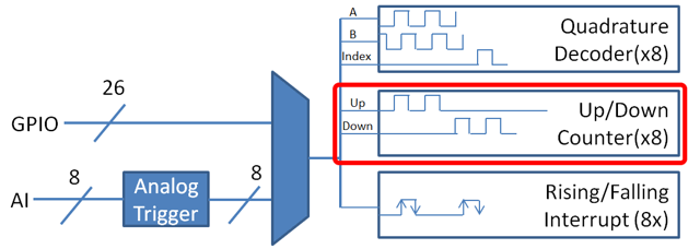
The Counter class (Java, C++) is a versatile class that allows the counting of pulse edges on a digital input. Counter is used as a component in several more-complicated WPILib classes (such as Encoder and Ultrasonic), but is also quite useful on its own.
Note
There are a total of 8 counter units in the roboRIO FPGA, meaning no more than 8 Counter objects may be instantiated at any one time, including those contained as resources in other WPILib objects. For detailed information on when a Counter may be used by another object, refer to the official API documentation.
Configuring a counter
The Counter class can be configured in a number of ways to provide differing functionalities.
Counter Modes
The Counter object may be configured to operate in one of four different modes:
Two-pulse mode: Counts up and down based on the edges of two different channels.
Semi-period mode: Measures the duration of a pulse on a single channel.
Pulse-length mode: Counts up and down based on the edges of one channel, with the direction determined by the duration of the pulse on that channel.
External direction mode: Counts up and down based on the edges of one channel, with a separate channel specifying the direction.
Note
In all modes except semi-period mode, the counter can be configured to increment either once per edge (2X decoding), or once per pulse (1X decoding). By default, counters are set to two-pulse mode, if only one channel is specified, the counter will only count up.
In two-pulse mode, the Counter will count up for every edge/pulse on the specified “up channel,” and down for every edge/pulse on the specified “down channel.” A counter can be initialized in two-pulse with the following code:
// Create a new Counter object in two-pulse mode
Counter counter = new Counter(Counter.Mode.k2Pulse);

@Override
public void robotInit() {
    // Set up the input channels for the counter
    counter.setUpSource(1);
    counter.setDownSource(2);

    // Set the decoding type to 2X
    counter.setUpSourceEdge(true, true);
    counter.setDownSourceEdge(true, true);
}
// Create a new Counter object in two-pulse mode
frc::Counter counter{frc::Counter::Mode::k2Pulse};

void Robot::RobotInit() {
    // Set up the input channels for the counter
    counter.SetUpSource(1);
    counter.SetDownSource(2);

    // Set the decoding type to 2X
    counter.SetUpSourceEdge(true, true);
    counter.SetDownSourceEdge(true, true);
In semi-period mode, the Counter will count the duration of the pulses on a channel, either from a rising edge to the next falling edge, or from a falling edge to the next rising edge. A counter can be initialized in semi-period mode with the following code:
// Create a new Counter object in two-pulse mode
Counter counter = new Counter(Counter.Mode.kSemiperiod);

@Override
public void robotInit() {
    // Set up the input channel for the counter
    counter.setUpSource(1);

    // Set the encoder to count pulse duration from rising edge to falling edge
    counter.setSemiPeriodMode(true);
}
// Create a new Counter object in two-pulse mode
frc::Counter counter{frc::Counter::Mode::kSemiperiod};

void Robot() {
    // Set up the input channel for the counter
    counter.SetUpSource(1);

    // Set the encoder to count pulse duration from rising edge to falling edge
    counter.SetSemiPeriodMode(true);
To get the pulse width, call the getPeriod() method:
// Return the measured pulse width in seconds
counter.getPeriod();
// Return the measured pulse width in seconds
counter.GetPeriod();
In pulse-length mode, the counter will count either up or down depending on the length of the pulse. A pulse below the specified threshold time will be interpreted as a forward count and a pulse above the threshold is a reverse count. This is useful for some gear tooth sensors which encode direction in this manner. A counter can be initialized in this mode as follows:
// Create a new Counter object in two-pulse mode
Counter counter = new Counter(Counter.Mode.kPulseLength);

@Override
public void robotInit() {
    // Set up the input channel for the counter
    counter.setUpSource(1);

    // Set the decoding type to 2X
    counter.setUpSourceEdge(true, true);

    // Set the counter to count down if the pulses are longer than .05 seconds
    counter.setPulseLengthMode(.05)
}
// Create a new Counter object in two-pulse mode
frc::Counter counter{frc::Counter::Mode::kPulseLength};

void Robot::RobotInit() {
    // Set up the input channel for the counter
    counter.SetUpSource(1);

    // Set the decoding type to 2X
    counter.SetUpSourceEdge(true, true);

    // Set the counter to count down if the pulses are longer than .05 seconds
    counter.SetPulseLengthMode(.05)
In external direction mode, the counter counts either up or down depending on the level on the second channel. If the direction source is low, the counter will increase, if the direction source is high, the counter will decrease (to reverse this, see the next section). A counter can be initialized in this mode as follows:
// Create a new Counter object in two-pulse mode
Counter counter = new Counter(Counter.Mode.kExternalDirection);

@Override
public void robotInit() {
    // Set up the input channels for the counter
    counter.setUpSource(1);
    counter.setDownSource(2);

    // Set the decoding type to 2X
    counter.setUpSourceEdge(true, true);
}
// Create a new Counter object in two-pulse mode
frc::Counter counter{frc::Counter::Mode::kExternalDirection};

void RobotInit() {
    // Set up the input channels for the counter
    counter.SetUpSource(1);
    counter.SetDownSource(2);

    // Set the decoding type to 2X
    counter.SetUpSourceEdge(true, true);
Configuring counter parameters
Note
The Counter class does not make any assumptions about units of distance; it will return values in whatever units were used to calculate the distance-per-pulse value. Users thus have complete control over the distance units used. However, units of time are always in seconds.
Note
The number of pulses used in the distance-per-pulse calculation does not depend on the decoding type - each “pulse” should always be considered to be a full cycle (rising and falling).
Apart from the mode-specific configurations, the Counter class offers a number of additional configuration methods:
// Configures the counter to return a distance of 4 for every 256 pulses
// Also changes the units of getRate
counter.setDistancePerPulse(4./256.);

// Configures the counter to consider itself stopped after .1 seconds
counter.setMaxPeriod(.1);

// Configures the counter to consider itself stopped when its rate is below 10
counter.setMinRate(10);

// Reverses the direction of the counter
counter.setReverseDirection(true);

// Configures an counter to average its period measurement over 5 samples
// Can be between 1 and 127 samples
counter.setSamplesToAverage(5);
// Configures the counter to return a distance of 4 for every 256 pulses
// Also changes the units of getRate
counter.SetDistancePerPulse(4./256.);

// Configures the counter to consider itself stopped after .1 seconds
counter.SetMaxPeriod(.1);

// Configures the counter to consider itself stopped when its rate is below 10
counter.SetMinRate(10);

// Reverses the direction of the counter
counter.SetReverseDirection(true);

// Configures an counter to average its period measurement over 5 samples
// Can be between 1 and 127 samples
counter.SetSamplesToAverage(5);
Reading information from counters
Regardless of mode, there is some information that the Counter class always exposes to users:
Count
Users can obtain the current count with the get() method:
// returns the current count
counter.get();
// returns the current count
counter.Get();
Distance
Note
Counters measure relative distance, not absolute; the distance value returned will depend on the position of the encoder when the robot was turned on or the encoder value was last reset.
If the distance per pulse has been configured, users can obtain the total distance traveled by the counted sensor with the getDistance() method:
// returns the current distance
counter.getDistance();
// returns the current distance
counter.GetDistance();
Note
Units of time for the Counter class are always in seconds.
Users can obtain the current rate of change of the counter with the getRate() method:
// Gets the current rate of the counter
counter.getRate();
// Gets the current rate of the counter
counter.GetRate();
Stopped
Users can obtain whether the counter is stationary with the getStopped() method:
// Gets whether the counter is stopped
counter.getStopped();
// Gets whether the counter is stopped
counter.GetStopped();
Users can obtain the direction in which the counter last moved with the getDirection() method:
// Gets the last direction in which the counter moved
counter.getDirection();
// Gets the last direction in which the counter moved
counter.GetDirection();
Period
Note
In semi-period mode, this method returns the duration of the pulse, not of the period.
Users can obtain the duration (in seconds) of the most-recent period with the getPeriod() method:
// returns the current period in seconds
counter.getPeriod();
// returns the current period in seconds
counter.GetPeriod();
Resetting a counter
To reset a counter to a distance reading of zero, call the reset() method. This is useful for ensuring that the measured distance corresponds to the actual desired physical measurement.
// Resets the encoder to read a distance of zero
counter.reset();
// Resets the encoder to read a distance of zero
counter.Reset();
Using counters in code
Counters are useful for a wide variety of robot applications - but since the Counter class is so varied, it is difficult to provide a good summary of them here. Many of these applications overlap with the Encoder class - a simple counter is often a cheaper alternative to a quadrature encoder. For a summary of potential uses for encoders in code, see Encoders - Software.
Encoders - Software
Note
This section covers encoders in software. For a hardware guide to encoders, see Encoders - Hardware.
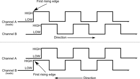
Encoders are devices used to measure motion (usually, the rotation of a shaft). The encoders used in FRC® are known as “quadrature encoders.” These encoders produce square-wave signals on two channels that are a quarter-period out-of-phase (hence the term, “quadrature”). The pulses are used to measure the rotation, and the direction of motion can be determined from which channel “leads” the other.
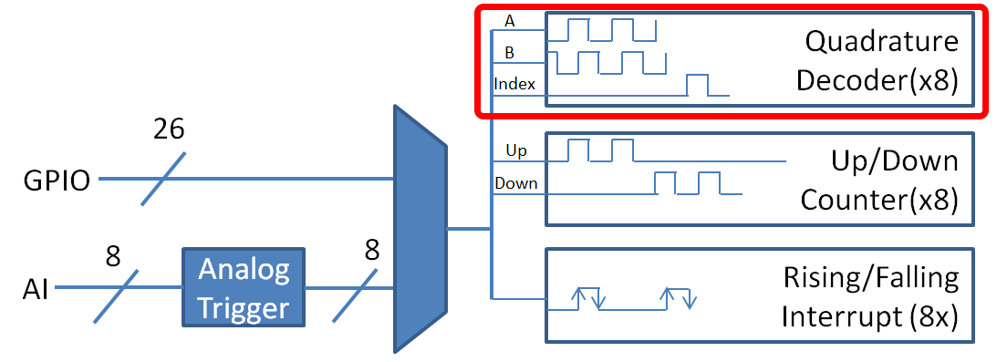
The FPGA handles encoders either through a counter module or an encoder module, depending on the decoding type - the choice is handled automatically by WPILib. The FPGA contains 8 encoder modules.
The Encoder class
WPILib provides support for encoders through the Encoder class (Java, C++). This class provides a simple API for configuring and reading data from encoders.
Important
The Encoder class is only used for encoders that are plugged directly into the roboRIO! Please reference the appropriate vendors’ documentation for using encoders plugged into motor controllers.
Initializing an encoder
An encoder can be instantiated as follows:
// Initializes an encoder on DIO pins 0 and 1
// Defaults to 4X decoding and non-inverted
Encoder encoder = new Encoder(0, 1);
// Initializes an encoder on DIO pins 0 and 1
// Defaults to 4X decoding and non-inverted
frc::Encoder encoder{0, 1};
The WPILib Encoder class can decode encoder signals in three different modes:
1X Decoding: Increments the distance for every complete period of the encoder signal (once per four edges).
2X Decoding: Increments the distance for every half-period of the encoder signal (once per two edges).
4X Decoding: Increments the distance for every edge of the encoder signal (four times per period).
4X decoding offers the greatest precision, but at the potential cost of increased “jitter” in rate measurements. To use a different decoding type, use the following constructor:
// Initializes an encoder on DIO pins 0 and 1
// 2X encoding and non-inverted
Encoder encoder = new Encoder(0, 1, false, Encoder.EncodingType.k2X);
// Initializes an encoder on DIO pins 0 and 1
// 2X encoding and non-inverted
frc::Encoder encoder{0, 1, false, frc::Encoder::EncodingType::k2X};
Configuring encoder parameters
Note
The Encoder class does not make any assumptions about units of distance; it will return values in whatever units were used to calculate the distance-per-pulse value. Users thus have complete control over the distance units used. However, units of time are always in seconds.
Note
The number of pulses used in the distance-per-pulse calculation does not depend on the decoding type - each “pulse” should always be considered to be a full cycle (four edges).
The Encoder class offers a number of configuration methods:
// Configures the encoder to return a distance of 4 for every 256 pulses
// Also changes the units of getRate
encoder.setDistancePerPulse(4./256.);
// Configures the encoder to consider itself stopped after .1 seconds
encoder.setMaxPeriod(.1);
// Configures the encoder to consider itself stopped when its rate is below 10
encoder.setMinRate(10);
// Reverses the direction of the encoder
encoder.setReverseDirection(true);
// Configures an encoder to average its period measurement over 5 samples
// Can be between 1 and 127 samples
encoder.setSamplesToAverage(5);
// Configures the encoder to return a distance of 4 for every 256 pulses
// Also changes the units of getRate
encoder.SetDistancePerPulse(4./256.);
// Configures the encoder to consider itself stopped after .1 seconds
encoder.SetMaxPeriod(.1);
// Configures the encoder to consider itself stopped when its rate is below 10
encoder.SetMinRate(10);
// Reverses the direction of the encoder
encoder.SetReverseDirection(true);
// Configures an encoder to average its period measurement over 5 samples
// Can be between 1 and 127 samples
encoder.SetSamplesToAverage(5);
Reading information from encoders
The Encoder class provides a wealth of information to the user about the motion of the encoder.
Note
Quadrature encoders measure relative distance, not absolute; the distance value returned will depend on the position of the encoder when the robot was turned on or the encoder value was last reset.
Users can obtain the total distance traveled by the encoder with the getDistance() method:
// Gets the distance traveled
encoder.getDistance();
// Gets the distance traveled
encoder.GetDistance();
Note
Units of time for the Encoder class are always in seconds.
Users can obtain the current rate of change of the encoder with the getRate() method:
// Gets the current rate of the encoder
encoder.getRate();
// Gets the current rate of the encoder
encoder.GetRate();
Users can obtain whether the encoder is stationary with the getStopped() method:
// Gets whether the encoder is stopped
encoder.getStopped();
// Gets whether the encoder is stopped
encoder.GetStopped();
Users can obtain the direction in which the encoder last moved with the getDirection() method:
// Gets the last direction in which the encoder moved
encoder.getDirection();
// Gets the last direction in which the encoder moved
encoder.GetDirection();
Users can obtain the period of the encoder pulses (in seconds) with the getPeriod() method:
// Gets the current period of the encoder
encoder.getPeriod();
// Gets the current period of the encoder
encoder.GetPeriod();
Resetting an encoder
To reset an encoder to a distance reading of zero, call the reset() method. This is useful for ensuring that the measured distance corresponds to the actual desired physical measurement, and is often called during a homing routine:
// Resets the encoder to read a distance of zero
encoder.reset();
// Resets the encoder to read a distance of zero
encoder.Reset();
Using encoders in code
Encoders are some of the most useful sensors in FRC; they are very nearly a requirement to make a robot capable of nontrivially-automated actuations and movement. The potential applications of encoders in robot code are too numerous to summarize fully here, but a few basic examples are provided below:
Driving to a distance
Encoders can be used on a robot drive to create a simple “drive to distance” routine. This is very useful for robot autonomy:
// Creates an encoder on DIO ports 0 and 1
Encoder encoder = new Encoder(0, 1);
// Initialize motor controllers and drive
Spark left1 new Spark(0);
Spark left2 = new Spark(1);
Spark right1 = new Spark(2);
Spark right2 = new Spark(3);
MotorControllerGroup leftMotors = new MotorControllerGroup(left1, left2);
MotorControllerGroup rightMotors = new MotorControllerGroup(right1, right2);
DifferentialDrive drive = new DifferentialDrive(leftMotors, rightMotors);
@Override
public void robotInit() {
// Configures the encoder's distance-per-pulse
// The robot moves forward 1 foot per encoder rotation
// There are 256 pulses per encoder rotation
encoder.setDistancePerPulse(1./256.);
}
@Override
public void autonomousPeriodic() {
// Drives forward at half speed until the robot has moved 5 feet, then stops:
if(encoder.getDistance() < 5) {
drive.tankDrive(.5, .5);
} else {
drive.tankDrive(0, 0);
}
}
// Creates an encoder on DIO ports 0 and 1.
frc::Encoder encoder{0, 1};
// Initialize motor controllers and drive
frc::Spark left1{0};
frc::Spark left2{1};
frc::Spark right1{2};
frc::Spark right2{3};
frc::MotorControllerGroup leftMotors{left1, left2};
frc::MotorControllerGroup rightMotors{right1, right2};
frc::DifferentialDrive drive{leftMotors, rightMotors};
void Robot::RobotInit() {
// Configures the encoder's distance-per-pulse
// The robot moves forward 1 foot per encoder rotation
// There are 256 pulses per encoder rotation
encoder.SetDistancePerPulse(1./256.);
}
void Robot:AutonomousPeriodic() {
// Drives forward at half speed until the robot has moved 5 feet, then stops:
if(encoder.GetDistance() < 5) {
drive.TankDrive(.5, .5);
} else {
drive.TankDrive(0, 0);
}
}
Stabilizing heading
Warning
Like with all control loops, users should be careful to ensure that the sensor direction and the turning direction are consistent. If they are not, the loop will be unstable and the robot will turn wildly.
Encoders can be used to ensure that a robot drives straight in a manner quite similar to how it is done with a gyroscope. A simple implementation with a P loop is given below:
// The encoders for the drive
Encoder leftEncoder = new Encoder(0,1);
Encoder rightEncoder = new Encoder(2,3);
// The gain for a simple P loop
double kP = 1;
// Initialize motor controllers and drive
Spark left1 = new Spark(0);
Spark left2 = new Spark(1);
Spark right1 = new Spark(2);
Spark right2 = new Spark(3);
MotorControllerGroup leftMotors = new MotorControllerGroup(left1, left2);
MotorControllerGroup rightMotors = new MotorControllerGroup(right1, right2);
DifferentialDrive drive = new DifferentialDrive(leftMotors, rightMotors);
@Override
public void autonomousInit() {
// Configures the encoders' distance-per-pulse
// The robot moves forward 1 foot per encoder rotation
// There are 256 pulses per encoder rotation
leftEncoder.setDistancePerPulse(1./256.);
rightEncoder.setDistancePerPulse(1./256.);
}
@Override
public void autonomousPeriodic() {
// Assuming no wheel slip, the difference in encoder distances is proportional to the heading error
double error = leftEncoder.getDistance() - rightEncoder.getDistance();
// Drives forward continuously at half speed, using the encoders to stabilize the heading
drive.tankDrive(.5 + kP * error, .5 - kP * error);
}
// The encoders for the drive
frc::Encoder leftEncoder{0,1};
frc::Encoder rightEncoder{2,3};
// The gain for a simple P loop
double kP = 1;
// Initialize motor controllers and drive
frc::Spark left1{0};
frc::Spark left2{1};
frc::Spark right1{2};
frc::Spark right2{3};
frc::MotorControllerGroup leftMotors{left1, left2};
frc::MotorControllerGroup rightMotors{right1, right2};
frc::DifferentialDrive drive{leftMotors, rightMotors};
void Robot::AutonomousInit() {
// Configures the encoders' distance-per-pulse
// The robot moves forward 1 foot per encoder rotation
// There are 256 pulses per encoder rotation
leftEncoder.SetDistancePerPulse(1./256.);
rightEncoder.SetDistancePerPulse(1./256.);
}
void Robot::AutonomousPeriodic() {
// Assuming no wheel slip, the difference in encoder distances is proportional to the heading error
double error = leftEncoder.GetDistance() - rightEncoder.GetDistance();
// Drives forward continuously at half speed, using the encoders to stabilize the heading
drive.TankDrive(.5 + kP * error, .5 - kP * error);
}
More-advanced implementations can use more-complicated control loops. Closing a control loop on the encoder difference is roughly analogous to closing it on the heading error, and so PD loops are particularly effective.
PID Control
Encoders are particularly useful as inputs to PID controllers (the heading stabilization example above is a simple P loop).
Homing a mechanism
Since encoders measure relative distance, it is often important to ensure that their “zero-point” is in the right place. A typical way to do this is a “homing routine,” in which a mechanism is moved until it hits a known position (usually accomplished with a limit switch), or “home,” and then the encoder is reset. The following code provides a basic example:
Encoder encoder = new Encoder(0, 1);
Spark spark = new Spark(0);
// Limit switch on DIO 2
DigitalInput limit = new DigitalInput(2);
public void autonomousPeriodic() {
// Runs the motor backwards at half speed until the limit switch is pressed
// then turn off the motor and reset the encoder
if(!limit.get()) {
spark.set(-.5);
} else {
spark.set(0);
encoder.reset();
}
}
frc::Encoder encoder{0,1};
frc::Spark spark{0};
// Limit switch on DIO 2
frc::DigitalInput limit{2};
void AutonomousPeriodic() {
// Runs the motor backwards at half speed until the limit switch is pressed
// then turn off the motor and reset the encoder
if(!limit.Get()) {
spark.Set(-.5);
} else {
spark.Set(0);
encoder.Reset();
}
}
Analog Inputs - Software
Note
This section covers analog inputs in software. For a hardware guide to analog inputs, see Analog Inputs - Hardware.
The roboRIO’s FPGA supports up to 8 analog input channels that can be used to read the value of an analog voltage from a sensor. Analog inputs may be used for any sensor that outputs a simple voltage.
Analog inputs from the FPGA by default return a 12-bit integer proportional to the voltage, from 0 to 5 volts.
The AnalogInput class
Note
It is often more convenient to use the Analog Potentiometers wrapper class than to use AnalogInput directly, as it supports scaling to meaningful units.
Support for reading the voltages on the FPGA analog inputs is provided through the AnalogInput class (Java, C++).
Initializing an AnalogInput
An AnalogInput may be initialized as follows:
// Initializes an AnalogInput on port 0
AnalogInput analog = new AnalogInput(0);
// Initializes an AnalogInput on port 0
frc::AnalogInput analog{0};
Oversampling and Averaging
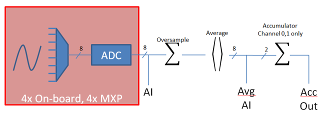
The FPGA’s analog input modules supports both oversampling and averaging. These behaviors are highly similar, but differ in a few important ways. Both may be used at the same time.
When oversampling is enabled, the FPGA will add multiple consecutive samples together, and return the accumulated value. Users may specify the number of bits of oversampling - for \(n\) bits of oversampling, the number of samples added together is \(2^{n}\):
// Sets the AnalogInput to 4-bit oversampling. 16 samples will be added together.
// Thus, the reported values will increase by about a factor of 16, and the update
// rate will decrease by a similar amount.
analog.setOversampleBits(4);
// Sets the AnalogInput to 4-bit oversampling. 16 samples will be added together.
// Thus, the reported values will increase by about a factor of 16, and the update
// rate will decrease by a similar amount.
analog.SetOversampleBits(4);
Averaging behaves much like oversampling, except the accumulated values are divided by the number of samples so that the scaling of the returned values does not change. This is often more-convenient, but occasionally the additional roundoff error introduced by the rounding is undesirable.
// Sets the AnalogInput to 4-bit averaging. 16 samples will be averaged together.
// The update rate will decrease by a factor of 16.
analog.setAverageBits(4);
// Sets the AnalogInput to 4-bit averaging. 16 samples will be averaged together.
// The update rate will decrease by a factor of 16.
analog.SetAverageBits(4);
Note
When oversampling and averaging are used at the same time, the oversampling is applied first, and then the oversampled values are averaged. Thus, 2-bit oversampling and 2-bit averaging used at the same time will increase the scale of the returned values by approximately a factor of 2, and decrease the update rate by approximately a factor of 4.
Reading values from an AnalogInput
Values can be read from an AnalogInput with one of four different methods:
The getValue method returns the raw instantaneous measured value from the analog input, without applying any calibration and ignoring oversampling and averaging settings. The returned value is an integer.
analog.getValue();
analog.GetValue();
The getVoltage method returns the instantaneous measured voltage from the analog input. Oversampling and averaging settings are ignored, but the value is rescaled to represent a voltage. The returned value is a double.
analog.getVoltage();
analog.GetVoltage();
The getAverageValue method returns the averaged value from the analog input. The value is not rescaled, but oversampling and averaging are both applied. The returned value is an integer.
analog.getAverageValue();
analog.GetAverageValue();
The getAverageVoltage method returns the averaged voltage from the analog input. Rescaling, oversampling, and averaging are all applied. The returned value is a double.
analog.getAverageVoltage();
analog.GetAverageVoltage();
Accumulator
Note
The accumulator methods do not currently support returning a value in units of volts - the returned value will always be an integer (specifically, a long).
Analog input channels 0 and 1 additionally support an accumulator, which integrates (adds up) the signal indefinitely, so that the returned value is the sum of all past measured values. Oversampling and averaging are applied prior to accumulation.
// Sets the initial value of the accumulator to 0
// This is the "starting point" from which the value will change over time
analog.setAccumulatorInitialValue(0);
// Sets the "center" of the accumulator to 0. This value is subtracted from
// all measured values prior to accumulation.
analog.setAccumulatorCenter(0);
// Returns the number of accumulated samples since the accumulator was last started/reset
analog.getAccumulatorCount();
// Returns the value of the accumulator. Return type is long.
analog.getAccumulatorValue();
// Resets the accumulator to the initial value
analog.resetAccumulator();
// Sets the initial value of the accumulator to 0
// This is the "starting point" from which the value will change over time
analog.SetAccumulatorInitialValue(0);
// Sets the "center" of the accumulator to 0. This value is subtracted from
// all measured values prior to accumulation.
analog.SetAccumulatorCenter(0);
// Returns the number of accumulated samples since the accumulator was last started/reset
analog.GetAccumulatorCount();
// Returns the value of the accumulator. Return type is long.
analog.GetAccumulatorValue();
// Resets the accumulator to the initial value
analog.ResetAccumulator();
Sometimes, it is necessarily to obtain matched measurements of the count and the value. This can be done using the getAccumulatorOutput method:
// Instantiate an AccumulatorResult object to hold the matched measurements
AccumulatorResult result = new AccumulatorResult();
// Fill the AccumulatorResult with the matched measurements
analog.getAccumulatorOutput(result);
// Read the values from the AccumulatorResult
long count = result.count;
long value = result.value;
// The count and value variables to fill
int_64t count;
int_64t value;
// Fill the count and value variables with the matched measurements
analog.GetAccumulatorOutput(count, value);
Using analog inputs in code
The AnalogInput class can be used to write code for a wide variety of sensors (including potentiometers, accelerometers, gyroscopes, ultrasonics, and more) that return their data as an analog voltage. However, if possible it is almost always more convenient to use one of the other existing WPILib classes that handles the lower-level code (reading the analog voltages and converting them to meaningful units) for you. Users should only directly use AnalogInput as a “last resort.”
Accordingly, for examples of how to effectively use analog sensors in code, users should refer to the other pages of this chapter that deal with more-specific classes.
Analog Potentiometers - Software
Note
This section covers analog potentiometers in software. For a hardware guide to analog potentiometers, see Analog Potentiometers - Hardware.
Potentiometers are variable resistors that allow information about position to be converted into an analog voltage signal. This signal can be read by the roboRIO to control whatever device is attached to the potentiometer.
While it is possible to read information from a potentiometer directly with an Analog Inputs - Software, WPILib provides an AnalogPotentiometer class (Java, C++) that handles re-scaling the values into meaningful units for the user. It is strongly encouraged to use this class.
In fact, the AnalogPotentiometer name is something of a misnomer - this class should be used for the vast majority of sensors that return their signal as a simple, linearly-scaled analog voltage.
The AnalogPotentiometer class
Note
The “full range” or “scale” parameters in the AnalogPotentiometer constructor are scale factors from a range of 0-1 to the actual range, not from 0-5. That is, they represent a native fractional scale, rather than a voltage scale.
An AnalogPotentiometer can be initialized as follows:
// Initializes an AnalogPotentiometer on analog port 0
// The full range of motion (in meaningful external units) is 0-180 (this could be degrees, for instance)
// The "starting point" of the motion, i.e. where the mechanism is located when the potentiometer reads 0v, is 30.
AnalogPotentiometer pot = new AnalogPotentiometer(0, 180, 30);
// Initializes an AnalogPotentiometer on analog port 0
// The full range of motion (in meaningful external units) is 0-180 (this could be degrees, for instance)
// The "starting point" of the motion, i.e. where the mechanism is located when the potentiometer reads 0v, is 30.
frc::AnalogPotentiometer pot{0, 180, 30};
Customizing the underlying AnalogInput
Note
If the user changes the scaling of the AnalogInput with oversampling, this must be reflected in the scale setting passed to the AnalogPotentiometer.
If the user would like to apply custom settings to the underlying AnalogInput used by the AnalogPotentiometer, an alternative constructor may be used in which the AnalogInput is injected:
// Initializes an AnalogInput on port 0, and enables 2-bit averaging
AnalogInput input = new AnalogInput(0);
input.setAverageBits(2);
// Initializes an AnalogPotentiometer with the given AnalogInput
// The full range of motion (in meaningful external units) is 0-180 (this could be degrees, for instance)
// The "starting point" of the motion, i.e. where the mechanism is located when the potentiometer reads 0v, is 30.
AnalogPotentiometer pot = new AnalogPotentiometer(input, 180, 30);
// Initializes an AnalogInput on port 0, and enables 2-bit averaging
frc::AnalogInput input{0};
input.SetAverageBits(2);
// Initializes an AnalogPotentiometer with the given AnalogInput
// The full range of motion (in meaningful external units) is 0-180 (this could be degrees, for instance)
// The "starting point" of the motion, i.e. where the mechanism is located when the potentiometer reads 0v, is 30.
frc::AnalogPotentiometer pot{input, 180, 30};
Reading values from the AnalogPotentiometer
The scaled value can be read by simply calling the get method:
pot.get();
pot.Get();
Using AnalogPotentiometers in code
Analog sensors can be used in code much in the way other sensors that measure the same thing can be. If the analog sensor is a potentiometer measuring an arm angle, it can be used similarly to an encoder. If it is an ultrasonic sensor, it can be used similarly to other ultrasonics.
It is very important to keep in mind that actual, physical potentiometers generally have a limited range of motion. Safeguards should be present in both the physical mechanism and the code to ensure that the mechanism does not break the sensor by traveling past its maximum throw.
Digital Inputs - Software
Note
This section covers digital inputs in software. For a hardware guide to digital inputs, see Digital Inputs - Hardware.
The roboRIO’s FPGA supports up to 26 digital inputs. 10 of these are made available through the built-in DIO ports on the RIO itself, while the other 16 are available through the MXP breakout port.
Digital inputs read one of two states - “high” or “low.” By default, the built-in ports on the RIO will read “high” due to internal pull-up resistors (for more information, see Digital Inputs - Hardware). Accordingly, digital inputs are most-commonly used with switches of some sort. Support for this usage is provided through the DigitalInput class (Java, C++).
The DigitalInput class
A DigitalInput can be initialized as follows:
// Initializes a DigitalInput on DIO 0
DigitalInput input = new DigitalInput(0);
// Initializes a DigitalInput on DIO 0
frc::DigitalInput input{0};
Reading the value of the DigitalInput
The state of the DigitalInput can be polled with the get method:
// Gets the value of the digital input. Returns true if the circuit is open.
input.get();
// Gets the value of the digital input. Returns true if the circuit is open.
input.Get();
Creating a DigitalInput from an AnalogInput
Note
An AnalogTrigger constructed with a port number argument can share that analog port with a separate AnalogInput, but two AnalogInput objects may not share the same port.
Sometimes, it is desirable to use an analog input as a digital input. This can be easily achieved using the AnalogTrigger class (Java, C++).
An AnalogTrigger may be initialized as follows. As with AnalogPotentiometer, an AnalogInput may be passed explicitly if the user wishes to customize the sampling settings:
// Initializes an AnalogTrigger on port 0
AnalogTrigger trigger0 = new AnalogTrigger(0);
// Initializes an AnalogInput on port 1 and enables 2-bit oversampling
AnalogInput input = new AnalogInput(1);
input.setAverageBits(2);
// Initializes an AnalogTrigger using the above input
AnalogTrigger trigger1 = new AnalogTrigger(input);
// Initializes an AnalogTrigger on port 0
frc::AnalogTrigger trigger0{0};
// Initializes an AnalogInput on port 1 and enables 2-bit oversampling
frc::AnalogInput input{1};
input.SetAverageBits(2);
// Initializes an AnalogTrigger using the above input
frc::AnalogTrigger trigger1{input};
Setting the trigger points
Note
For details on the scaling of “raw” AnalogInput values, see Analog Inputs - Software.
To convert the analog signal to a digital one, it is necessary to specify at what values the trigger will enable and disable. These values may be different to avoid “dithering” around the transition point:
// Sets the trigger to enable at a raw value of 3500, and disable at a value of 1000
trigger.setLimitsRaw(1000, 3500);
// Sets the trigger to enable at a voltage of 4 volts, and disable at a value of 1.5 volts
trigger.setLimitsVoltage(1.5, 4);
// Sets the trigger to enable at a raw value of 3500, and disable at a value of 1000
trigger.SetLimitsRaw(1000, 3500);
// Sets the trigger to enable at a voltage of 4 volts, and disable at a value of 1.5 volts
trigger.SetLimitsVoltage(1.5, 4);
Using DigitalInputs in code
As almost all switches on the robot will be used through a DigitalInput, this class is extremely important for effective robot control.
Limiting the motion of a mechanism
Nearly all motorized mechanisms (such as arms and elevators) in FRC® should be given some form of “limit switch” to prevent them from damaging themselves at the end of their range of motions. A short example is given below:
Spark spark = new Spark(0);
// Limit switch on DIO 2
DigitalInput limit = new DigitalInput(2);
public void autonomousPeriodic() {
// Runs the motor forwards at half speed, unless the limit is pressed
if(!limit.get()) {
spark.set(.5);
} else {
spark.set(0);
}
}
// Motor for the mechanism
frc::Spark spark{0};
// Limit switch on DIO 2
frc::DigitalInput limit{2};
void AutonomousPeriodic() {
// Runs the motor forwards at half speed, unless the limit is pressed
if(!limit.Get()) {
spark.Set(.5);
} else {
spark.Set(0);
}
}
Homing a mechanism
Limit switches are very important for being able to “home” a mechanism with a encoder. For an example of this, see Homing a mechanism.
Programming Limit Switches
Limit switches are often used to control mechanisms on robots. While limit switches are simple to use, they only can sense a single position of a moving part. This makes them ideal for ensuring that movement doesn’t exceed some limit but not so good at controlling the speed of the movement as it approaches the limit. For example, a rotational shoulder joint on a robot arm would best be controlled using a potentiometer or an absolute encoder, the limit switch could make sure that if the potentiometer ever failed, the limit switch would stop the robot from going to far and causing damage.
Limit switches can have “normally open” or “normally closed” outputs. This will control if a high signal means the switch is opened or closed. To learn more about limit switch hardware see this article.
Controlling a Motor with Two Limit Switches
DigitalInput toplimitSwitch = new DigitalInput(0);
DigitalInput bottomlimitSwitch = new DigitalInput(1);
PWMVictorSPX motor = new PWMVictorSPX(0);
Joystick joystick = new Joystick(0);
@Override
public void teleopPeriodic() {
setMotorSpeed(joystick.getRawAxis(2));
}
public void setMotorSpeed(double speed) {
if (speed > 0) {
if (toplimitSwitch.get()) {
// We are going up and top limit is tripped so stop
motor.set(0);
} else {
// We are going up but top limit is not tripped so go at commanded speed
motor.set(speed);
}
} else {
if (bottomlimitSwitch.get()) {
// We are going down and bottom limit is tripped so stop
motor.set(0);
} else {
// We are going down but bottom limit is not tripped so go at commanded speed
motor.set(speed);
}
}
}
frc::DigitalInput toplimitSwitch {0};
frc::DigitalInput bottomlimitSwitch {1};
frc::PWMVictorSPX motor {0};
frc::Joystick joystick {0};
void TeleopPeriodic() {
SetMotorSpeed(joystick.GetRawAxis(2));
}
void SetMotorSpeed(double speed) {
if (speed > 0) {
if (toplimitSwitch.Get()) {
// We are going up and top limit is tripped so stop
motor.Set(0);
} else {
// We are going up but top limit is not tripped so go at commanded speed
motor.Set(speed);
}
} else {
if (bottomlimitSwitch.Get()) {
// We are going down and bottom limit is tripped so stop
motor.Set(0);
} else {
// We are going down but bottom limit is not tripped so go at commanded speed
motor.Set(speed);
}
}
}
Miscellaneous Hardware APIs
This section highlights miscellaneous hardware APIs that are standalone.
Addressable LEDs
LED strips have been commonly used by teams for several years for a variety of reasons. They allow teams to debug robot functionality from the audience, provide a visual marker for their robot, and can simply add some visual appeal. WPILib has an API for controlling WS2812 LEDs with their data pin connected via PWM.
Instantiating the AddressableLED Object
You first create an AddressableLED object that takes the PWM port as an argument. It must be a PWM header on the roboRIO. Then you set the number of LEDs located on your LED strip, with can be done with the setLength() function.
Important
It is important to note that setting the length of the LED header is an expensive task and it’s not recommended to run this periodically.
After the length of the strip has been set, you’ll have to create an AddressableLEDBuffer object that takes the number of LEDs as an input. You’ll then call myAddressableLed.setData(myAddressableLEDBuffer) to set the led output data. Finally, you can call myAddressableLed.start() to write the output continuously. Below is a full example of the initialization process.
Note
C++ does not have an AddressableLEDBuffer, and instead uses an Array.
17 @Override
18 public void robotInit() {
19 // PWM port 9
20 // Must be a PWM header, not MXP or DIO
21 m_led = new AddressableLED(9);
22
23 // Reuse buffer
24 // Default to a length of 60, start empty output
25 // Length is expensive to set, so only set it once, then just update data
26 m_ledBuffer = new AddressableLEDBuffer(60);
27 m_led.setLength(m_ledBuffer.getLength());
28
29 // Set the data
30 m_led.setData(m_ledBuffer);
31 m_led.start();
32 }
11class Robot : public frc::TimedRobot {
12 static constexpr int kLength = 60;
13
14 // PWM port 9
15 // Must be a PWM header, not MXP or DIO
16 frc::AddressableLED m_led{9};
17 std::array<frc::AddressableLED::LEDData, kLength>
18 m_ledBuffer; // Reuse the buffer
19 // Store what the last hue of the first pixel is
20 int firstPixelHue = 0;
38 void RobotInit() override {
39 // Default to a length of 60, start empty output
40 // Length is expensive to set, so only set it once, then just update data
41 m_led.SetLength(kLength);
42 m_led.SetData(m_ledBuffer);
43 m_led.Start();
44 }
Setting the Entire Strip to One Color
Color can be set to an individual led on the strip using two methods. setRGB() which takes RGB values as an input and setHSV() which takes HSV values as an input.
Using RGB Values
RGB stands for Red, Green, and Blue. This is a fairly common color model as it’s quite easy to understand. LEDs can be set with the setRGB method that takes 4 arguments: index of the LED, amount of red, amount of green, amount of blue. The amount of Red, Green, and Blue are integer values between 0-255.
for (var i = 0; i < m_ledBuffer.getLength(); i++) {
// Sets the specified LED to the RGB values for red
m_ledBuffer.setRGB(i, 255, 0, 0);
}
m_led.setData(m_ledBuffer);
for (int i = 0; i < kLength; i++) {
m_ledBuffer[i].SetRGB(255, 0, 0);
}
m_led.SetData(m_ledBuffer);
Using HSV Values
HSV stands for Hue, Saturation, and Value. Hue describes the color or tint, saturation being the amount of gray, and value being the brightness. In WPILib, Hue is an integer from 0 - 180. Saturation and Value are integers from 0 - 255. If you look at a color picker like Google’s, Hue will be 0 - 360 and Saturation and Value are from 0% to 100%. This is the same way that OpenCV handles HSV colors. Make sure the HSV values entered to WPILib are correct, or the color produced might not be the same as was expected.
LEDs can be set with the setHSV method that takes 4 arguments: index of the LED, hue, saturation, and value. An example is shown below for setting the color of an LED strip to red (hue of 0).
for (var i = 0; i < m_ledBuffer.getLength(); i++) {
// Sets the specified LED to the HSV values for red
m_ledBuffer.setHSV(i, 0, 100, 100);
}
m_led.setData(m_ledBuffer);
for (int i = 0; i < kLength; i++) {
m_ledBuffer[i].SetHSV(0, 100, 100);
}
m_led.SetData(m_ledBuffer);
Creating a Rainbow Effect
The below method does a couple of important things. Inside of the for loop, it equally distributes the hue over the entire length of the strand and stores the individual LED hue to a variable called hue. Then the for loop sets the HSV value of that specified pixel using the hue value.
Moving outside of the for loop, the m_rainbowFirstPixelHue then iterates the pixel that contains the “initial” hue creating the rainbow effect. m_rainbowFirstPixelHue then checks to make sure that the hue is inside the hue boundaries of 180. This is because HSV hue is a value from 0-180.
Note
It’s good robot practice to keep the robotPeriodic() method as clean as possible, so we’ll create a method for handling setting our LED data. We’ll call this method rainbow() and call it from robotPeriodic().
42 private void rainbow() {
43 // For every pixel
44 for (var i = 0; i < m_ledBuffer.getLength(); i++) {
45 // Calculate the hue - hue is easier for rainbows because the color
46 // shape is a circle so only one value needs to precess
47 final var hue = (m_rainbowFirstPixelHue + (i * 180 / m_ledBuffer.getLength())) % 180;
48 // Set the value
49 m_ledBuffer.setHSV(i, hue, 255, 128);
50 }
51 // Increase by to make the rainbow "move"
52 m_rainbowFirstPixelHue += 3;
53 // Check bounds
54 m_rainbowFirstPixelHue %= 180;
55 }
23 void Rainbow() {
24 // For every pixel
25 for (int i = 0; i < kLength; i++) {
26 // Calculate the hue - hue is easier for rainbows because the color
27 // shape is a circle so only one value needs to precess
28 const auto pixelHue = (firstPixelHue + (i * 180 / kLength)) % 180;
29 // Set the value
30 m_ledBuffer[i].SetHSV(pixelHue, 255, 128);
31 }
32 // Increase by to make the rainbow "move"
33 firstPixelHue += 3;
34 // Check bounds
35 firstPixelHue %= 180;
36 }
Now that we have our rainbow method created, we have to actually call the method and set the data of the LED.
34 @Override
35 public void robotPeriodic() {
36 // Fill the buffer with a rainbow
37 rainbow();
38 // Set the LEDs
39 m_led.setData(m_ledBuffer);
40 }
46 void RobotPeriodic() override {
47 // Fill the buffer with a rainbow
48 Rainbow();
49 // Set the LEDs
50 m_led.SetData(m_ledBuffer);
51 }
52};
Motor Controllers
A motor controller is responsible on your robot for making motors move. For brushed DC motors such as CIMs or 775s, the motor controller regulates the voltage that the motor receives, much like a light bulb. For brushless motor controllers such as the Spark MAX, the controller regulates the power delivered to each “phase” of the motor.
Note
Another name for a motor controller is a speed controller.
Hint
One can make a quick, non-competition-legal motor controller by removing the motor from a cordless BRUSHED drill and attaching PowerPoles or equivalents to the motor’s leads. Make sure that the voltage supplied by the drill will not damage the motor, but note that the 775 is fine at up to 24 volts.
Warning
Connecting a BRUSHLESS motor controller straight to power, such as to a conventional brushed motor controller, will destroy the motor!
FRC Legal Motor Controllers
Motor controllers come in lots of shapes, sizes and feature sets. This is the full list of FRC® Legal motor controllers as of 2022:
DMC 60/DMC 60c Motor Controller (P/N: 410-334-1, 410-334-2)
Jaguar Motor Controller (P/N: MDL-BDC, MDL-BDC24, and 217-3367) connected to PWM only
Nidec Dynamo BLDC Motor with Controller to control integral actuator only (P/N 840205-000, am-3740)
SD540 Motor Controller (P/N: SD540x1, SD540x2, SD540x4, SD540Bx1, SD540Bx2, SD540Bx4, SD540C)
Spark Motor Controller (P/N: REV-11-1200)
Spark MAX Motor Controller (P/N: REV-11-2158)
Talon FX Motor Controller (P/N: 217-6515, 19-708850, am-6515, am-6515_Short) for controlling integral Falcon 500 only
Talon Motor Controller (P/N: CTRE_Talon, CTRE_Talon_SR, and am-2195)
Talon SRX Motor Controller (P/N: 217-8080, am-2854, 14-838288)
Venom Motor with Controller (P/N BDC-10001) for controlling integral motor only
Victor 884 Motor Controller (P/N: VICTOR-884-12/12)
Victor 888 Motor Controller (P/N: 217-2769)
Victor SP Motor Controller (P/N: 217-9090, am-2855, 14-868380)
Victor SPX Motor Controller (P/N: 217-9191, 17-868388, am-3748)
Pneumatics
Pneumatics are a quick and easy way to make something that’s in one state or another using compressed air. For information on operating pneumatics, see Operating pneumatic cylinders.
FRC Legal Pneumatics controllers
Pneumatics Control Module (P/N: am-2858, 217-4243)
Pneumatic Hub (P/N REV-11-1852)
Relays
A relay controls power to a motor or custom electronics in an On/Off fashion.
FRC Legal Relay Modules
Spike H-Bridge Relay (P/N: 217-0220 and SPIKE-RELAY-H)
Automation Direct Relay (P/N: AD-SSR6M12-DC200D, AD-SSR6M25-DC200D, AD-SSR6M40-DC200D)
Power Distribution Hub (PDH) switched channel (P/N REV-11-1850)
CAN Devices
Using CAN Devices
CAN has many advantages over other methods of connection between the robot controller and peripheral devices.
CAN connections are daisy-chained from device to device, which often results in much shorter wire runs than having to wire each device to the RIO itself.
Much more data can be sent over a CAN connection than over a PWM connection - thus, CAN motor controllers are capable of a much more expansive feature-set than are PWM motor controllers.
CAN is bi-directional, so CAN motor controllers can send data back to the RIO, again facilitating a more expansive feature-set than can be offered by PWM Controllers.
For instructions on wiring CAN devices, see the relevant section of the robot wiring guide.
CAN devices generally have their own WPILib classes. The following sections will describe the use of several of these classes.
Pneumatics Control Module
The Pneumatics Control Module (PCM) is a CAN-based device that provides complete control over the compressor and up to 8 solenoids per module. The PCM is integrated into WPILib through a series of classes that make it simple to use.
The closed loop control of the Compressor and Pressure switch is handled by the Compressor class (Java, C++), and the Solenoids are handled by the Solenoid (Java, C++) and DoubleSolenoid (Java, C++) classes.
An additional PCM module can be used where the modules corresponding solenoids are differentiated by the module number in the constructors of the Solenoid and Compressor classes.
For more information on controlling the compressor, see Operating a Compressor for Pneumatics.
For more information on controlling solenoids, see Operating Pneumatic Cylinders.
Pneumatic Hub
The Pneumatic Hub (PH) is a CAN-based device that provides complete control over the compressor and up to 16 solenoids per module. The PH is integrated into WPILib through a series of classes that make it simple to use.
The closed loop control of the Compressor and Pressure switch is handled by the Compressor class (Java, C++), and the Solenoids are handled by the Solenoid (Java, C++) and DoubleSolenoid (Java, C++) classes.
An additional PH module can be used where the modules corresponding solenoids are differentiated by the module number in the constructors of the Solenoid and Compressor classes.
For more information on controlling the compressor, see Operating a Compressor for Pneumatics.
For more information on controlling solenoids, see Operating Pneumatic Cylinders.
Power Distribution Module
The CTRE Power Distribution Panel (PDP) and Rev Power Distribution Hub (PDH) can use their CAN connectivity to communicate a wealth of status information regarding the robot’s power use to the roboRIO, for use in user code. This has the capability to report current temperature, the bus voltage, the total robot current draw, the total robot energy use, and the individual current draw of each device power channel. This data can be used for a number of advanced control techniques, such as motor torque limiting and brownout avoidance.
Creating a Power Distribution Object
To use the either Power Distribution module, create an instance of the PowerDistribution class (Java, C++). With no arguments, the Power Distribution object will be detected, and must use CAN ID of 0 for CTRE or 1 for REV. If the CAN ID is non-default, additional constructors are available to specify the CAN ID and type.
PowerDistribution examplePD = new PowerDistribution();
PowerDistribution examplePD = new PowerDistribution(0, ModuleType.kCTRE);
PowerDistribution examplePD = new PowerDistribution(1, ModuleType.kRev);
PowerDistribution examplePD{};
PowerDistribution examplePD{0, frc::PowerDistribution::ModuleType::kCTRE};
PowerDistribution examplePD{1, frc::PowerDistribution::ModuleType::kRev};
Note: it is not necessary to create a PowerDistribution object unless you need to read values from it. The board will work and supply power on all the channels even if the object is never created.
Warning
To enable voltage and current logging in the Driver Station, the CAN ID for the CTRE Power Distribution Panel must be 0, and for the REV Power Distribution Hub it must be 1.
Reading the Bus Voltage
double voltage = examplePD.getVoltage();
double voltage = examplePD.GetVoltage();
Monitoring the bus voltage can be useful for (among other things) detecting when the robot is near a brownout, so that action can be taken to avoid brownout in a controlled manner. See the roboRIO Brownouts document for more information.
Reading the Temperature
double temp = examplePD.getTemperature();
double temp = examplePD.GetTemperature();
Monitoring the temperature can be useful for detecting if the robot has been drawing too much power and needs to be shut down for a while, or if there is a short or other wiring problem.
Reading the Total Current, Power, and Energy
double current = examplePD.getTotalCurrent();
double power = examplePD.getTotalPower();
double energy = examplePD.getTotalEnergy();
double current = examplePD.GetTotalCurrent();
double power = examplePD.GetTotalPower();
double energy = examplePD.GetTotalEnergy();
Monitoring the total current, power and energy can be useful for controlling how much power is being drawn from the battery, both for preventing brownouts and ensuring that mechanisms have sufficient power available to perform the actions required. Power is the bus voltage multiplied by the current with the units Watts. Energy is the power summed over time with units Joules.
Reading Individual Channel Currents
The PDP/PDH also allows users to monitor the current drawn by the individual device power channels. You can read the current on any of the 16 PDP channels (0-15) or 24 PDH channels (0-23). For example, to read the current on channel 0:
double current = examplePD.getCurrent(0);
double current = examplePD.GetCurrent(0);
Monitoring individual device current draws can be useful for detecting shorts or stalled motors.
Using the Switchable Channel (PDH)
The REV PDH has one channel that can be switched on or off to control custom circuits.
examplePD.setSwitchableChannel(true);
examplePD.setSwitchableChannel(false);
examplePD.SetSwitchableChannel(true);
examplePD.SetSwitchableChannel(false);
Third-Party CAN Devices
A number of FRC® vendors offer their own CAN peripherals. As CAN devices offer expansive feature-sets, vendor CAN devices require similarly expansive code libraries to operate. As a result, these libraries are not maintained as an official part of WPILib, but are instead maintained by the vendors themselves. For a guide to installing third-party libraries, see 3rd Party Libraries
A list of common third-party CAN devices from various vendors, along with links to corresponding external documentation, is provided below:
Cross-the-Road Electronics
Cross-the-Road Electronics (CTRE) offers several CAN peripherals with external libraries. General resources for all CTRE devices include:
CTRE Motor Controllers
Talon FX (with Falcon 500 Motor)
Talon SRX
Victor SPX
CTRE Sensors
CANcoder
Pigeon IMU
CANifier
REV Robotics
REV Robotics currently offers the SPARK MAX motor controller, which has a similar feature-set to the Talon SRX.
REV Motor Controllers
SPARK MAX
FRC CAN Device Specifications
This document seeks to describe the basic functions of the current FRC® CAN system and the requirements for any new CAN devices seeking to work with the system.
Addressing
FRC CAN nodes assign arbitration IDs based on a pre-defined scheme that breaks the ID into 5 components:
Device Type
This is a 5-bit value describing the type of device being addressed. A
table of currently assigned device types can be found below. If you wish
to have a new device type assigned from the Reserved pool, please
submit a request to FIRST.
Device Types |
|
|---|---|
Broadcast Messages |
0 |
Robot Controller |
1 |
Motor Controller |
2 |
Relay Controller |
3 |
Gyro Sensor |
4 |
Accelerometer |
5 |
Ultrasonic Sensor |
6 |
Gear Tooth Sensor |
7 |
Power Distribution Module |
8 |
Pneumatics Controller |
9 |
Miscellaneous |
10 |
IO Breakout |
11 |
Reserved |
12-30 |
Firmware Update |
31 |
Manufacturer
This is an 8-bit value indicating the manufacturer of the CAN device.
Currently assigned values can be found in the table below. If you wish
to have a manufacturer ID assigned from the Reservedpool, please
submit a request to FIRST.
Manufacturer |
|
|---|---|
Broadcast |
0 |
NI |
1 |
Luminary Micro |
2 |
DEKA |
3 |
CTR Electronics |
4 |
REV Robotics |
5 |
Grapple |
6 |
MindSensors |
7 |
Team Use |
8 |
Kauai Labs |
9 |
Copperforge |
10 |
Playing With Fusion |
11 |
Studica |
12 |
Reserved |
13-255 |
API/Message Identifier
The API or Message Identifier is a 10-bit value that identifies a
particular command or message type. These identifiers are unique for
each Manufacturer + Device Type combination (so an API identifier that
may be a “Voltage Set” for a Luminary Micro Motor Controller may be a
“Status Get” for a CTR Electronics Motor Controller or Current Get
for a CTR Power Distribution Module).
The Message identifier is further broken down into 2 sub-fields: the 6-bit API Class and the 4-bit API Index.
API Class
The API Class is a 6-bit identifier for an API grouping. Similar messages are grouped into a single API Class. An example of the API Classes for the Jaguar Motor Controller is shown in the table below.
API Class |
|
|---|---|
Voltage Control Mode |
0 |
Speed Control Mode |
1 |
Voltage Compensation Mode |
2 |
Position Control Mode |
3 |
Current Control Mode |
4 |
Status |
5 |
Periodic Status |
6 |
Configuration |
7 |
Ack |
8 |
API Index
The API Index is a 4-bit identifier for a particular message within an API Class. An example of the API Index values for the Jaguar Motor Controller Speed Control API Class is shown in the table below.
API Index |
|
|---|---|
Enable Control |
0 |
Disable Control |
1 |
Set Setpoint |
2 |
P Constant |
3 |
I Constant |
4 |
D Constant |
5 |
Set Reference |
6 |
Trusted Enable |
7 |
Trusted Set No Ack |
8 |
Trusted Set Setpoint No Ack |
10 |
Set Setpoint No Ack |
11 |
Device Number
Device Number is a 6-bit quantity indicating the number of the device of a particular type. Devices should default to device ID 0 to match other components of the FRC Control System. Device 0x3F may be reserved for device specific broadcast messages.
Protected Frames
FRC CAN Nodes which implement actuator control capability (motor controllers, relays, pneumatics controllers, etc.) must implement a way to verify that the robot is enabled and that commands originate with the main robot controller (i.e. the roboRIO).
Broadcast Messages
Broadcast messages are messages sent to all nodes by setting the device type and manufacturer fields to 0. The API Class for broadcast messages is 0. The currently defined broadcast messages are shown in the table below:
Description |
|
|---|---|
Disable |
0 |
System Halt |
1 |
System Reset |
2 |
Device Assign |
3 |
Device Query |
4 |
Heartbeat |
5 |
Sync |
6 |
Update |
7 |
Firmware Version |
8 |
Enumerate |
9 |
System Resume |
10 |
Devices should disable immediately when receiving the Disable message (arbID 0), implementation of other broadcast messages is optional.
Requirements for FRC CAN Nodes
For CAN Nodes to be accepted for use in the FRC System, they must:
Communicate using Arbitration IDs which match the prescribed FRC format:
A valid, issued CAN Device Type (per Table 1 - CAN Device Types)
A valid, issued Manufacturer ID (per Table 2 - CAN Manufacturer Codes)
API Class(es) and Index(s) assigned and documented by the device manufacturer
A user selectable device number if multiple units of the device type are intended to co-exist on the same network.
Support the minimum Broadcast message requirements as detailed in the Broadcast Messages section.
If controlling actuators, utilize a scheme to assure that the robot is issuing commands, is enabled, and is still present
Provide software library support for LabVIEW, C++, and Java or arrange with FIRST® or FIRSTs Control System Partners to provide such interfaces.
Universal Heartbeat
The roboRIO provides a universal CAN heartbeat that any device on the bus can listen and react to. This heartbeat is sent every 20ms. The heartbeat has a full CAN ID of 0x01011840 (which is the NI Manufacturer ID, RobotController type, Device ID 0 and API ID 0x062). It is an 8 byte CAN packet. The important byte in here is byte 5 (index 4). The layout is the following bitfield.
Description |
Width |
|---|---|
RedAlliance |
1 |
Enabled |
1 |
Autonomous |
1 |
Test |
1 |
WatchdogEnabled |
1 |
Reserved |
3 |
The flag to watch for is WatchdogEnabled. If that flag is set, that means motor controllers are enabled.
If 100ms has passed since this packet was received, the robot program can be considered hung, and devices should act as if the robot has been disabled.
Basic Programming
Git Version Control Introduction
Important
A more in-depth guide on Git is available on the Git website.
Git is a Distributed Version Control System (VCS) created by Linus Torvalds, also known for creating and maintaining the Linux kernel. Version Control is a system for tracking changes of code for developers. The advantages of Git Version Control are:
Separate testing environments into branches
Ability to navigate to a particular commit without removing history
Ability to manage commits in various ways, including combining them
Various other features, see here
Prerequisites
Important
This tutorial uses the Windows operating system
You have to download and install Git from the following links:
Note
You may need to add Git to your path
Git Vocabulary
Git revolves around several core commands:
Repository: the data structure of your code, including a
.gitfolder in the root directoryCommit: a particular saved state of the repository, this includes all files and additions
Branch: a means of separating various commits, having a unique history. This is primarily used for separating development and stable branches.
Push: update the remote repository with your local changes
Pull: update your local repository with the remote changes
Clone: retrieving a local copy of a repository to modify
Fork: duplicating a pre-existing repository to modify, and to compare against the original
Merge: combining various changes from different branches/commits/forks into a single history
Repository
A Git repository is a data structure containing the structure, history, and files of a project.
Git repositories usually consist of:
A
.gitfolder. This folder contains the various information about the repository.A
.gitignorefile. This file contains the files or directories that you do not want included when you commit.Files and folders. This is the main content of the repository.
Creating the repository
You can store the repository locally, or through a remote. A remote being the cloud, or possibly another storage medium that hosts your repository. GitHub is a popular free hosting service. Numerous developers use it, and that’s what this tutorial will use.
Note
There are various providers that can host repositories. Gitlab and Bitbucket are a few alternatives to Github.
Creating a GitHub Account
Go ahead and create a GitHub account by visiting the website and following the own screen prompts.

Local Creation
After creating and verifying your account, you’ll want to visit the homepage. It’ll look similar to the shown image.
Click the plus icon in the top right.
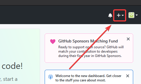
Then click “New Repository”
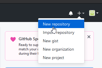
Fill out the appropriate information, and then click “Create repository”
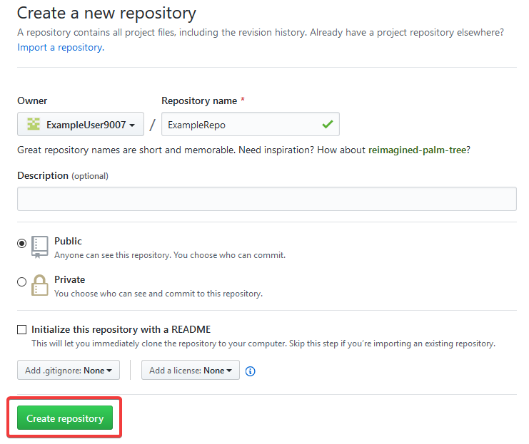
You should see a screen similar to this
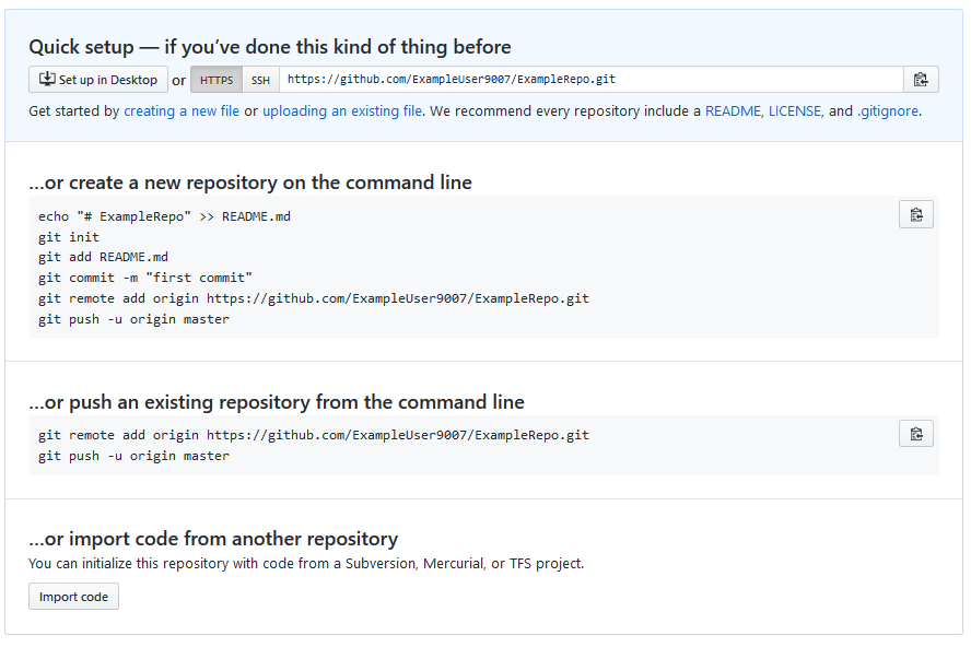
Note
The keyboard shortcut Ctrl+~ can be used to open a terminal in Visual Studio Code.
Now you’ll want to open a PowerShell window and navigate to your project directory. An excellent tutorial on PowerShell can be found here. Please consult your search engine on how to open a terminal on alternative operating systems.
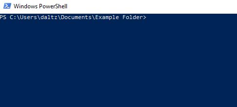
If a directory is empty, a file needs to be created in order for git to have something to track. In the below Empty Directory example, we created a file called README.md with the contents of # Example Repo. For FRC® Robot projects, the below Existing Project commands should be run in the root of a project created by the VS Code WPILib Project Creator. More details on the various commands can be found in the subsequent sections.
Note
Replace the filepath "C:\Users\ExampleUser9007\Documents\Example Folder" with the one you want to create the repo in, and replace the remote URL https://github.com/ExampleUser9007/ExampleRepo.git with the URL for the repo you created in the previous steps.
> cd "C:\Users\ExampleUser9007\Documents\Example Folder"
> git init
Initialized empty Git repository in C:/Users/ExampleUser9007/Documents/Example Folder/.git/
> echo "# ExampleRepo" >> README.md
> git add README.md
> git commit -m "First commit"
[main (root-commit) fafafa] First commit
1 file changed, 1 insertions(+), 0 deletions(-)
create mode 100644 README.md
> git remote add origin https://github.com/ExampleUser9007/ExampleRepo.git
> git push -u origin main
> cd "C:\Users\ExampleUser9007\Documents\Example Folder"
> git init
Initialized empty Git repository in C:/Users/ExampleUser9007/Documents/Example Folder/.git/
> git add .
> git commit -m "First commit"
[main (root-commit) fafafa] First commit
1 file changed, 1 insertions(+), 0 deletions(-)
create mode 100644 README.md
> git remote add origin https://github.com/ExampleUser9007/ExampleRepo.git
> git push -u origin main
Commits
Repositories are primarily composed of commits. Commits are saved states or versions of code.
In the previous example, we created a file called README.md. Open that file in your favorite text editor and edit a few lines. After tinkering with the file for a bit, simply save and close. Navigate to PowerShell and type the following commands.
> git add README.md
> git commit -m "Adds a description to the repository"
[main bcbcbc] Adds a description to the repository
1 file changed, 2 insertions(+), 0 deletions(-)
> git push
Note
Writing good commit messages is a key part of a maintainable project. A guide on writing commit messages can be found here.
Git Pull
Note
git fetch can be used when the user does not wish to automatically merge into the current working branch
This command retrieves the history or commits from the remote repository. When the remote contains work you do not have, it will attempt to automatically merge. See Merging.
Run: git pull
Git Add
This command adds a selected file(s) to a commit. To commit every file/folder that isn’t excluded via gitignore.
Run: git add FILENAME.txt where FILENAME.txt is the name and extension of the file to add to a commit.
Run: git add . will add every untracked, unexcluded file when ran in the root of the repository.
Git Commit
This command creates the commit and stores it locally. This saves the state and adds it to the repositories history.
Run: git commit -m "type message here"
Branches
Branches are a similar to parallel worlds to Git. They start off the same, and then they can “branch” out into different varying paths. Consider the Git control flow to look similar to this.

In the above example, main was branched (or duplicated) into the branch Feature 1 and someone checked out the branch, creating a local copy. Then, someone committed (or uploaded) their changes, merging them into the branch Feature 1. You are “merging” the changes from one branch into another.
Creating a Branch
Run: git branch branch-name where branch-name is the name of the branch to create. The new branch history will be created from the current active branch.
Entering a Branch
Once a branch is created, you have to then enter the branch.
Run: git checkout branch-name where branch-name is the branch that was previously created.
Merging
In scenarios where you want to copy one branches history into another, you can merge them. A merge is done by calling git merge branch-name with branch-name being the name of the branch to merge from. It is automatically merged in the current active branch.
It’s common for a remote repository to contain work (history) that you do not have. Whenever you run git pull, it will attempt to automatically merge those commits. That merge may look like the below.

However, in the above example, what if File 1 was modified by both branch FeatureA and FeatureB? This is called a merge conflict. A merge conflict will can be resolved by editing the conflicting file. In the example, we would need to edit File 1 to keep the history or changes that we want. After that has been done. Simply re-add, re-commit, and then push your changes.
Resets
Sometimes history needs to be reset, or a commit needs to be undone. This can be done multiple ways.
Reverting the Commit
Note
You cannot revert a merge, as git does not know which branch or origin it should choose.
To revert history leading up to a commit run git revert commit-id. The commit IDs can be shown using the git log command.
Resetting the Head
Warning
Forcibly resetting the head is a dangerous command. It permanently erases all history past the target. You have been warned!
Run: git reset --hard commit-id.
Forks
Forks can be treated similarly to branches. You can merge the upstream (original repository) into the origin (forked repository).
Cloning an Existing Repo
In the situation that a repository is already created and stored on a remote, you can clone it using
git clone https://github.com/myrepo.git
where myrepo.git is replaced with your git repo. If you follow this, you can skip to :ref:commits <docs/software/basic-programming/git-getting-started:Commits>`.
Updating a Fork
Add the upstream:
git remote add upstream https://github.com/ORIGINAL_OWNER/ORIGINAL_REPOSITORY.gitConfirm it was added via:
git remote -vPull changes from upstream:
git fetch upstreamMerge the changes into head:
git merge upstream/upstream-branch-name
Gitignore
Important
It is extremely important that teams do not modify the .gitignore file that is included with their robot project. This can lead to offline deployment not working.
A .gitignore file is commonly used as a list of files to not automatically commit with git add. Any files or directory listed in this file will not be committed. They will also not show up with git status.
Additional Information can be found here
Hiding a Folder
Simply add a new line containing the folder to hide, with a forward slash at the end
EX: directory-to-exclude/
Hiding a File
Add a new line with the name of the file to hide, including any prepending directory relative to the root of the repository.
EX: directory/file-to-hide.txt
EX: file-to-hide2.txt
Additional Information
A much more in-depth tutorial can be found at the official git website.
A guide for correcting common mistakes can be found at the git flight rules repository.
The C++ Units Library
WPILib is coupled with a Units library for C++ teams. This library leverages the C++ type system to enforce proper dimensionality for method parameters, automatically perform unit conversions, and even allow users to define arbitrary defined unit types. Since the C++ type system is enforced at compile-time, the library has essentially no runtime cost.
Using the Units Library
The units library is a header-only library. You must include the relevant header in your source files for the units you want to use. Here’s a list of available units.
#include <units/acceleration.h>
#include <units/angle.h>
#include <units/angular_acceleration.h>
#include <units/angular_velocity.h>
#include <units/area.h>
#include <units/capacitance.h>
#include <units/charge.h>
#include <units/concentration.h>
#include <units/conductance.h>
#include <units/current.h>
#include <units/curvature.h>
#include <units/data.h>
#include <units/data_transfer_rate.h>
#include <units/density.h>
#include <units/dimensionless.h>
#include <units/energy.h>
#include <units/force.h>
#include <units/frequency.h>
#include <units/illuminance.h>
#include <units/impedance.h>
#include <units/inductance.h>
#include <units/length.h>
#include <units/luminous_flux.h>
#include <units/luminous_intensity.h>
#include <units/magnetic_field_strength.h>
#include <units/magnetic_flux.h>
#include <units/mass.h>
#include <units/moment_of_inertia.h>
#include <units/power.h>
#include <units/pressure.h>
#include <units/radiation.h>
#include <units/solid_angle.h>
#include <units/substance.h>
#include <units/temperature.h>
#include <units/time.h>
#include <units/torque.h>
#include <units/velocity.h>
#include <units/voltage.h>
#include <units/volume.h>
The units/math.h header provides unit-aware functions like units::math::abs().
Unit Types and Container Types
The C++ units library is based around two sorts of type definitions: unit types and container types.
Unit Types
Unit types correspond to the abstract concept of a unit, without any actual stored value. Unit types are the fundamental “building block” of the units library - all unit types are defined constructively (using the compound_unit template) from a small number of “basic” unit types (such as meters, seconds, etc).
While unit types cannot contain numerical values, their use in building other unit types means that when a type or method uses a template parameter to specify its dimensionality, that parameter will be a unit type.
Container Types
Container types correspond to an actual quantity dimensioned according to some unit - that is, they are what actually hold the numerical value. Container types are constructed from unit types with the unit_t template. Most unit types have a corresponding container type that has the same name suffixed by _t - for example, the unit type units::meter corresponds to the container type units::meter_t.
Whenever a specific quantity of a unit is used (as a variable or a method parameter), it will be an instance of the container type. By default, container types will store the actual value as a double - advanced users may change this by calling the unit_t template manually.
A full list of unit and container types can be found in the documentation.
Creating Instances of Units
To create an instance of a specific unit, we create an instance of its container type:
// The variable speed has a value of 5 meters per second.
units::meter_per_second_t speed{5.0};
Alternatively, the units library has type literals defined for some of the more common container types. These can be used in conjunction with type inference via auto to define a unit more succinctly:
// The variable speed has a value of 5 meters per second.
auto speed = 5_mps;
Units can also be initialized using a value of an another container type, as long as the types can be converted between one another. For example, a meter_t value can be created from a foot_t value.
auto feet = 6_ft;
units::meter_t meters{feet};
In fact, all container types representing convertible unit types are implicitly convertible. Thus, the following is perfectly legal:
units::meter_t distance = 6_ft;
In short, we can use any unit of length in place of any other unit of length, anywhere in our code; the units library will automatically perform the correct conversion for us.
Performing Arithmetic with Units
Container types support all of the ordinary arithmetic operations of their underlying data type, with the added condition that the operation must be dimensionally sound. Thus, addition must always be performed on two compatible container types:
// Add two meter_t values together
auto sum = 5_m + 7_m; // sum is 12_m
// Adds meters to feet; both are length, so this is fine
auto sum = 5_m + 7_ft;
// Tries to add a meter_t to a second_t, will throw a compile-time error
auto sum = 5_m + 7_s;
Multiplication may be performed on any pair of container types, and yields the container type of a compound unit:
Note
When a calculation yields a compound unit type, this type will only be checked for validity at the point of operation if the result type is specified explicitly. If auto is used, this check will not occur. For example, when we divide distance by time, we may want to ensure the result is, indeed, a velocity (i.e. units::meter_per_second_t). If the return type is declared as auto, this check will not be made.
// Multiply two meter_t values, result is square_meter_t
auto product = 5_m * 7_m; // product is 35_sq_m
// Divide a meter_t value by a second_t, result is a meter_per_second_t
units::meter_per_second_t speed = 6_m / 0.5_s; // speed is 12_mps
<cmath> Functions
Some std functions (such as clamp) are templated to accept any type on which the arithmetic operations can be performed. Quantities stored as container types will work with these functions without issue.
However, other std functions work only on ordinary numerical types (e.g. double). The units library’s units::math namespace contains wrappers for several of these functions that accept units. Examples of such functions include sqrt, pow, etc.
auto area = 36_sq_m;
units::meter_t sideLength = units::math::sqrt(area);
Removing the Unit Wrapper
To convert a container type to its underlying value, use the value() method. This serves as an escape hatch from the units type system, which should be used only when necessary.
units::meter_t distance = 6.5_m;
double distanceMeters = distance.value();
Example of the Units Library in WPILib Code
Several arguments for methods in new features of WPILib (ex. kinematics) use the units library. Here is an example of sampling a trajectory.
// Sample the trajectory at 1.2 seconds. This represents where the robot
// should be after 1.2 seconds of traversal.
Trajectory::State point = trajectory.Sample(1.2_s);
// Since units of time are implicitly convertible, this is exactly equivalent to the above code
Trajectory::State point = trajectory.Sample(1200_ms);
Some WPILib classes represent objects that could naturally work with multiple choices of unit types - for example, a motion profile might operate on either linear distance (e.g. meters) or angular distance (e.g. radians). For such classes, the unit type is required as a template parameter:
// Creates a new set of trapezoidal motion profile constraints
// Max velocity of 10 meters per second
// Max acceleration of 20 meters per second squared
frc::TrapezoidProfile<units::meters>::Constraints{10_mps, 20_mps_sq};
// Creates a new set of trapezoidal motion profile constraints
// Max velocity of 10 radians per second
// Max acceleration of 20 radians per second squared
frc::TrapezoidProfile<units::radians>::Constraints{10_rad_per_s, 20__rad_per_s / 1_s};
For more detailed documentation, please visit the official GitHub page for the units library.
Joysticks
A joystick can be used with the Driver Station program to control the robot. Almost any “controller” that can be recognized by Windows can be used as a joystick. Joysticks are accessed using the GenericHID class. This class has three relevant subclasses for preconfigured joysticks. You may also implement your own for other controllers by extending GenericHID. The first is Joystick which is useful for standard flight joysticks. The second is XboxController which works for the Xbox 360, Xbox One, or Logitech F310 (in XInput mode). Finally, the PS4Controller class is ideal for using that controller. Each axis of the controller ranges from -1 to 1.
The command based way to use the these classes is detailed in the section: Binding Commands to Triggers
Driver Station Joysticks
The USB Devices Tab of the Driver Station is used to setup and configure the joystick for use with the robot. Pressing a button on a joystick will cause its entry in the table to light up green. Selecting the joystick will show the values of axes, buttons and the POV that can be used to determine the mapping between physical joystick features and axis or button numbers.
The USB Devices Tab also assigns a joystick index to each joystick. To reorder the joysticks simply click and drag. The Driver Station software will try to preserve the ordering of devices between runs. It is a good idea to note what order your devices should be in and check each time you start the Driver Station software that they are correct.
When the Driver Station is in disabled mode, it is routinely looking for status changes on the joystick devices. Unplugged devices are removed from the list and new devices are opened and added. When not connected to the FMS, unplugging a joystick will force the Driver Station into disabled mode. To start using the joystick again: plug the joystick in, check that it shows up in the right spot, then re-enable the robot. While the Driver Station is in enabled mode, it will not scan for new devices. This is a time consuming operation and timely update of signals from attached devices takes priority.
Note
For some joysticks the startup routine will read whatever position the joysticks are in as the center position, therefore, when the computer is turned on (or when the joystick is plugged in) the joysticks should be at their center position.
When the robot is connected to the Field Management System at competition, the Driver Station mode is dictated by the FMS. This means that you cannot disable your robot and the DS cannot disable itself in order to detect joystick changes. A manual complete refresh of the joysticks can be initiated by pressing the F1 key on the keyboard. Note that this will close and re-open all devices, so all devices should be in their center position as noted above.
Joystick Class
Joystick exampleJoystick = new Joystick(0); // 0 is the USB Port to be used as indicated on the Driver Station
Joystick exampleJoystick{0}; // 0 is the USB Port to be used as indicated on the Driver Station
The Joystick class is designed to make using a flight joystick to operate the robot significantly easier. Depending on the flight joystick, the user may need to set the specific X, Y, Z, and Throttle channels that your flight joystick uses. This class offers special methods for accessing the angle and magnitude of the flight joystick.
XboxController Class
XboxController exampleXbox = new XboxController(0); // 0 is the USB Port to be used as indicated on the Driver Station
XboxController exampleXbox{0}; // 0 is the USB Port to be used as indicated on the Driver Station
An example of how to use buttons on the XboxController.
39 private final XboxController m_joystick = new XboxController(0);
40 final JoystickButton l2 = new JoystickButton(m_joystick, 9);
41 final JoystickButton r2 = new JoystickButton(m_joystick, 10);
42 final JoystickButton l1 = new JoystickButton(m_joystick, 11);
43 final JoystickButton r1 = new JoystickButton(m_joystick, 12);
44 r1.whenPressed(new PrepareToPickup(m_claw, m_wrist, m_elevator));
45 r2.whenPressed(new Pickup(m_claw, m_wrist, m_elevator));
46 l1.whenPressed(new Place(m_claw, m_wrist, m_elevator));
47 l2.whenPressed(new Autonomous(m_drivetrain, m_claw, m_wrist, m_elevator));
41 frc2::JoystickButton(&m_joy, 9).WhenPressed(
42 Autonomous(m_claw, m_wrist, m_elevator, m_drivetrain));
43 frc2::JoystickButton(&m_joy, 10)
44 .WhenPressed(Pickup(m_claw, m_wrist, m_elevator));
45 frc2::JoystickButton(&m_joy, 11)
46 .WhenPressed(Place(m_claw, m_wrist, m_elevator));
47 frc2::JoystickButton(&m_joy, 12)
48 .WhenPressed(PrepareToPickup(m_claw, m_wrist, m_elevator));
The XboxController class provides named indicies for each of the buttons that you can access with XboxController.Button.kX.value. The rumble feature of the controller can be controlled by using XboxController.setRumble(GenericHID.RumbleType.kRightRumble, value). Many users do a split stick arcade drive that uses the left stick for just forwards / backwards and the right stick for left / right turning.
PS4Controller Class
PS4Controller examplePS4 = new PS4Controller(0); // 0 is the USB Port to be used as indicated on the Driver Station
PS4Controller examplePS4{0}; // 0 is the USB Port to be used as indicated on the Driver Station
The PS4Controller class provides named indicies for each of the buttons. These buttons can accessed with PS4Controller.Button.kSquare.value. The rumble feature of the controller can be controlled by using PS4Controller.setRumble(GenericHID.RumbleType.kRightRumble, value).
POV

On joysticks, the POV is a directional hat that can select one of 8 different angles or read -1 for unpressed. The XboxController D-pad works the same as a POV. Be careful when using a POV with exact angle requirements as it is hard for the user to ensure they select exactly the angle desired.
GenericHID Usage
An axis can be used with .getRawAxis(0) (if not using any of the classes above) that returns the current value. Zero and one in this example are each the index of an axis as found in the Driver Station mentioned above.
private final PWMSparkMax m_leftMotor = new PWMSparkMax(0);
private final PWMSparkMax m_rightMotor = new PWMSparkMax(1);
private final DifferentialDrive m_robotDrive = new DifferentialDrive(m_leftMotor, m_rightMotor);
private final GenericHID m_stick = new GenericHID(0);
m_robotDrive.arcadeDrive(-m_stick.getRawAxis(0), m_stick.getRawAxis(1));
frc::PWMVictorSPX m_leftMotor{0};
frc::PWMVictorSPX m_rightMotor{1};
frc::DifferentialDrive m_robotDrive{m_leftMotor, m_rightMotor};
frc::GenericHID m_stick{0};
m_robotDrive.ArcadeDrive(-m_stick.GetRawAxis(0), m_stick.GetRawAxis(1));
Button Usage
Unlike an axis, you will usually want to use the pressed and released methods to respond to button input. These will return true if the button has been activated since the last check. This is helpful for taking an action once when the event occurs but not having to continuously do it while the button is held down.
if (joystick.getRawButtonPressed(0)) {
turnIntakeOn(); // When pressed the intake turns on
}
if (joystick.getRawButtonReleased(0)) {
turnIntakeOff(); // When released the intake turns off
}
OR
if (joystick.getRawButton(0)) {
turnIntakeOn();
} else {
turnIntakeOff();
}
if (joystick.GetRawButtonPressed(0)) {
turnIntakeOn(); // When pressed the intake turns on
}
if (joystick.GetRawButtonReleased(0)) {
turnIntakeOff(); // When released the intake turns off
}
OR
if (joystick.GetRawButton(0)) {
turnIntakeOn();
} else {
turnIntakeOff();
}
A common request is to toggle something on and off with the press of a button. Toggles should be used with caution, as they require the user to keep track of the robot state.
boolean toggle = false;
if (joystick.getRawButtonPressed(0)) {
if (toggle) {
// Current state is true so turn off
retractIntake();
toggle = false;
} else {
// Current state is false so turn on
deployIntake();
toggle = true;
}
}
bool toggle{false};
if (joystick.GetRawButtonPressed(0)) {
if (toggle) {
// Current state is true so turn off
retractIntake();
toggle = false;
} else {
// Current state is false so turn on
deployIntake();
toggle = true;
}
}
Reading Stacktraces
An unexpected error has occurred.
When your robot code hits an unexpected error, you will see this message show up in some console output (Driver Station or RioLog). You’ll probably also notice your robot abruptly stop, or possibly never move. These unexpected errors are called unhandled exceptions.
When an unhandled exception occurs, it means that your code has one or more bugs which need to be fixed.
This article will explore some of the tools and techniques involved in finding and fixing those bugs.
What’s a “Stack Trace”?
The unexpected error has occurred message is a signal that a stack trace has been printed out.
In Java and C++, a stack data structure is used to store information about which function or method is currently being executed.
A stack trace prints information about what was on this stack when the unhandled exception occurred. This points you to the lines of code which were running just before the problem happened. While it doesn’t always point you to the exact root cause of your issue, it’s usually the best place to start looking.
What’s an “Unhandled Exception”?
An unrecoverable error is any condition which arises where the processor cannot continue executing code. It almost always implies that, even though the code compiled and started running, it no longer makes sense for execution to continue.
In almost all cases, the root cause of an unhandled exception is code that isn’t correctly implemented. It almost never implies that any hardware has malfunctioned.
So How Do I Fix My Issue?
Read the Stack Trace
To start, search above the unexpected error has occurred for the stack trace.
In Java, it should look something like this:
Error at frc.robot.Robot.robotInit(Robot.java:24): Unhandled exception: java.lang.NullPointerException
at frc.robot.Robot.robotInit(Robot.java:24)
at edu.wpi.first.wpilibj.TimedRobot.startCompetition(TimedRobot.java:94)
at edu.wpi.first.wpilibj.RobotBase.runRobot(RobotBase.java:335)
at edu.wpi.first.wpilibj.RobotBase.lambda$startRobot$0(RobotBase.java:387)
at java.base/java.lang.Thread.run(Thread.java:834)
There’s a few important things to pick out of here:
There was an
ErrorThe error was due to an
Unhandled exceptionThe exception was a
java.lang.NullPointerExceptionThe error happened while running line
24inside ofRobot.javarobotInitwas the name of the method executing when the error happened.
robotInitis a function in thefrc.robot.Robotpackage (AKA, your team’s code)robotInitwas called from a number of functions from theedu.wpi.first.wpilibjpackage (AKA, the WPILib libraries)
The list of indented lines starting with the word at represent the state of the stack at the time the error happened. Each line represents one method, which was called by the method right below it.
For example, If the error happened deep inside your codebase, you might see more entries on the stack:
Error at frc.robot.Robot.buggyMethod(TooManyBugs.java:1138): Unhandled exception: java.lang.NullPointerException
at frc.robot.Robot.buggyMethod(TooManyBugs.java:1138)
at frc.robot.Robot.barInit(Bar.java:21)
at frc.robot.Robot.fooInit(Foo.java:34)
at frc.robot.Robot.robotInit(Robot.java:24)
at edu.wpi.first.wpilibj.TimedRobot.startCompetition(TimedRobot.java:94)
at edu.wpi.first.wpilibj.RobotBase.runRobot(RobotBase.java:335)
at edu.wpi.first.wpilibj.RobotBase.lambda$startRobot$0(RobotBase.java:387)
at java.base/java.lang.Thread.run(Thread.java:834)
In this case: robotInit called fooInit, which in turn called barInit, which in turn called buggyMethod. Then, during the execution of buggyMethod, the NullPointerException occurred.
Java will usually produce stack traces automatically when programs run into issues. C++ will require more digging to extract the same info. Usually, a single-step debugger will need to be hooked up to the executing robot program.
Stack traces can be found in the debugger tab of VS Code:
Stack traces in C++ will generally look similar to this:
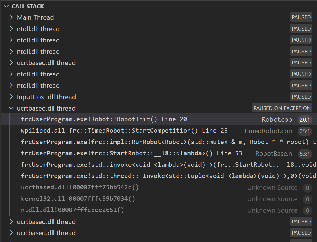
There’s a few important things to pick out of here:
The code execution is currently paused.
The reason it paused was one thread having an
exceptionThe error happened while running line
20inside ofRobot.cppRobotInitwas the name of the method executing when the error happened.
RobotInitis a function in theRobot::namespace (AKA, your team’s code)RobotInitwas called from a number of functions from thefrc::namespace (AKA, the WPILib libraries)
This “call stack” window represents the state of the stack at the time the error happened. Each line represents one method, which was called by the method right below it.
The examples in this page assume you are running code examples in simulation, with the debugger connected and watching for unexpected errors. Similar techniques should apply while running on a real robot.
Perform Code Analysis
Once you’ve found the stack trace, and found the lines of code which are triggering the unhandled exception, you can start the process of determining root cause.
Often, just looking in (or near) the problematic location in code will be fruitful. You may notice things you forgot, or lines which don’t match an example you’re referencing.
Note
Developers who have lots of experience working with code will often have more luck looking at code than newer folks. That’s ok, don’t be discouraged! The experience will come with time.
A key strategy for analyzing code is to ask the following questions:
When was the last time the code “worked” (IE, didn’t have this particular error)?
What has changed in the code between the last working version, and now?
Frequent testing and careful code changes help make this particular strategy more effective.
Run the Single Step Debugger
Sometimes, just looking at code isn’t enough to spot the issue. The single-step debugger is a great option in this case - it allows you to inspect the series of events leading up to the unhandled exception.
Search for More Information
Google is a phenomenal resource for understanding the root cause of errors. Searches involving the programming language and the name of the exception will often yield good results on more explanations for what the error means, how it comes about, and potential fixes.
Seeking Outside Help
If all else fails, you can seek out advice and help from others (both in-person and online). When working with folks who aren’t familiar with your codebase, it’s very important to provide the following information:
Access to your source code, (EX: on github.com)
The full text of the error, including the full stack trace.
Common Examples & Patterns
There are a number of common issues which result in runtime exceptions.
Null Pointers and References
Both C++ and Java have the concept of “null” - they use it to indicate something which has not yet been initialized, and does not refer to anything meaningful.
Manipulating a “null” reference will produce a runtime error.
For example, consider the following code:
19 PWMSparkMax armMotorCtrl;
20
21 @Override
22 public void robotInit() {
23 armMotorCtrl.setInverted(true);
24 }
17class Robot : public frc::TimedRobot {
18 public:
19 void RobotInit() override {
20 motorRef->SetInverted(false);
21 }
22
23 private:
24 frc::PWMVictorSPX m_armMotor{0};
25 frc::PWMVictorSPX* motorRef;
26};
When run, you’ll see output that looks like this:
********** Robot program starting **********
Error at frc.robot.Robot.robotInit(Robot.java:23): Unhandled exception: java.lang.NullPointerException
at frc.robot.Robot.robotInit(Robot.java:23)
at edu.wpi.first.wpilibj.TimedRobot.startCompetition(TimedRobot.java:107)
at edu.wpi.first.wpilibj.RobotBase.runRobot(RobotBase.java:373)
at edu.wpi.first.wpilibj.RobotBase.startRobot(RobotBase.java:463)
at frc.robot.Main.main(Main.java:23)
Warning at edu.wpi.first.wpilibj.RobotBase.runRobot(RobotBase.java:388): The robot program quit unexpectedly. This is usually due to a code error.
The above stacktrace can help determine where the error occurred.
See https://wpilib.org/stacktrace for more information.
Error at edu.wpi.first.wpilibj.RobotBase.runRobot(RobotBase.java:395): The startCompetition() method (or methods called by it) should have handled the exception above.
Reading the stack trace, you can see that the issue happened inside of the robotInit() function, on line 23, and the exception involved “Null Pointer”.
By going to line 23, you can see there is only one thing which could be null - armMotorCtrl. Looking further up, you can see that the armMotorCtrl object is declared, but never instantiated.
Alternatively, you can step through lines of code with the single step debugger, and stop when you hit line 23. Inspecting the armMotorCtrl object at that point would show that it is null.
Exception has occurred: W32/0xc0000005
Unhandled exception thrown: read access violation.
this->motorRef was nullptr.
In Simulation, this will show up in a debugger window that points to line 20 in the above buggy code.
You can view the full stack trace by clicking the debugger tab in VS Code:
The error is specific - our member variable motorRef was declared, but never assigned a value. Therefore, when we attempt to use it to call a method using the -> operator, the exception occurs.
The exception states its type was nullptr.
Fixing Null Object Issues
Generally, you will want to ensure each reference has been initialized before using it. In this case, there is a missing line of code to instantiate the armMotorCtrl before calling the setInverted() method.
A functional implementation could look like this:
19 PWMSparkMax armMotorCtrl;
20
21 @Override
22 public void robotInit() {
23 armMotorCtrl = new PWMSparkMax(0);
24 armMotorCtrl.setInverted(true);
25 }
17class Robot : public frc::TimedRobot {
18 public:
19 void RobotInit() override {
20 motorRef = &m_armMotor;
21 motorRef->SetInverted(false);
22 }
23
24 private:
25 frc::PWMVictorSPX m_armMotor{0};
26 frc::PWMVictorSPX* motorRef;
27};
Divide by Zero
It is not generally possible to divide an integer by zero, and expect reasonable results. Most processors (including the roboRIO) will raise an Unhandled Exception.
For example, consider the following code:
18 int armLengthRatio;
19 int elbowToWrist_in = 39;
20 int shoulderToElbow_in = 0; //TODO
21
22 @Override
23 public void robotInit() {
24 armLengthRatio = elbowToWrist_in / shoulderToElbow_in;
25 }
17 class Robot : public frc::TimedRobot {
18 public:
19 void RobotInit() override {
20 armLengthRatio = elbowToWrist_in / shoulderToElbow_in;
21 }
22
23 private:
24 int armLengthRatio;
25 int elbowToWrist_in = 39;
26 int shoulderToElbow_in = 0; //TODO
27
28 };
When run, you’ll see output that looks like this:
********** Robot program starting **********
Error at frc.robot.Robot.robotInit(Robot.java:24): Unhandled exception: java.lang.ArithmeticException: / by zero
at frc.robot.Robot.robotInit(Robot.java:24)
at edu.wpi.first.wpilibj.TimedRobot.startCompetition(TimedRobot.java:107)
at edu.wpi.first.wpilibj.RobotBase.runRobot(RobotBase.java:373)
at edu.wpi.first.wpilibj.RobotBase.startRobot(RobotBase.java:463)
at frc.robot.Main.main(Main.java:23)
Warning at edu.wpi.first.wpilibj.RobotBase.runRobot(RobotBase.java:388): The robot program quit unexpectedly. This is usually due to a code error.
The above stacktrace can help determine where the error occurred.
See https://wpilib.org/stacktrace for more information.
Error at edu.wpi.first.wpilibj.RobotBase.runRobot(RobotBase.java:395): The startCompetition() method (or methods called by it) should have handled the exception above.
Looking at the stack trace, we can see a java.lang.ArithmeticException: / by zero exception has occurred on line 24. If you look at the two variables which are used on the right-hand side of the = operator, you might notice one of them has been initialized to zero. Looks like someone forgot to update it! Furthermore, the zero-value variable is used in the denominator of a division operation. Hence, the divide by zero error happens.
Alternatively, by running the single-step debugger and stopping on line 24, you could inspect the value of all variables to discover shoulderToElbow_in has a value of 0.
Exception has occurred: W32/0xc0000094
Unhandled exception at 0x00007FF71B223CD6 in frcUserProgram.exe: 0xC0000094: Integer division by zero.
In Simulation, this will show up in a debugger window that points to line 20 in the above buggy code.
You can view the full stack trace by clicking the debugger tab in VS Code:
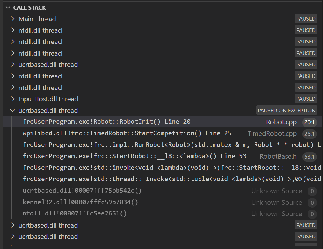
Looking at the message, we see the error is described as Integer division by zero. If you look at the two variables which are used on the right-hand side of the = operator on line 20, you might notice one of them has been initialized to zero. Looks like someone forgot to update it! Furthermore, the zero-value variable is used in the denominator of a division operation. Hence, the divide by zero error happens.
Note that the error messages might look slightly different on the roboRIO, or on an operating system other than windows.
Fixing Divide By Zero Issues
Divide By Zero issues can be fixed in a number of ways. It’s important to start by thinking about what a zero in the denominator of your calculation _means_. Is it plausible? Why did it happen in the particular case you saw?
Sometimes, you just need to use a different number other than 0.
A functional implementation could look like this:
18 int armLengthRatio;
19 int elbowToWrist_in = 39;
20 int shoulderToElbow_in = 3;
21
22 @Override
23 public void robotInit() {
24
25 armLengthRatio = elbowToWrist_in / shoulderToElbow_in;
26
27 }
17 class Robot : public frc::TimedRobot {
18 public:
19 void RobotInit() override {
20 armLengthRatio = elbowToWrist_in / shoulderToElbow_in;
21 }
22
23 private:
24 int armLengthRatio;
25 int elbowToWrist_in = 39;
26 int shoulderToElbow_in = 3
27
28 };
Alternatively, if zero is a valid value, adding if/else statements around the calculation can help you define alternate behavior to avoid making the processor perform a division by zero.
Finally, changing variable types to be float or double can help you get around the issue - floating-point numbers have special values like NaN to represent the results of a divide-by-zero operation. However, you may still have to handle this in code which consumes that calculation’s value.
HAL Resource Already Allocated
A very common FRC-specific error occurs when the code attempts to put two hardware-related on the same HAL resource (usually, roboRIO IO pin.)
For example, consider the following code:
19 PWMSparkMax leftFrontMotor;
20 PWMSparkMax leftRearMotor;
21
22 @Override
23 public void robotInit() {
24 leftFrontMotor = new PWMSparkMax(0);
25 leftRearMotor = new PWMSparkMax(0);
26 }
17class Robot : public frc::TimedRobot {
18 public:
19 void RobotInit() override {
20 m_frontLeftMotor.Set(0.5);
21 m_rearLeftMotor.Set(0.25);
22 }
23
24 private:
25 frc::PWMVictorSPX m_frontLeftMotor{0};
26 frc::PWMVictorSPX m_rearLeftMotor{0};
27
28 };
When run, you’ll see output that looks like this:
********** Robot program starting **********
Error at frc.robot.Robot.robotInit(Robot.java:25): Unhandled exception: edu.wpi.first.hal.util.AllocationException: Code: -1029
PWM or DIO 0 previously allocated.
Location of the previous allocation:
at frc.robot.Robot.robotInit(Robot.java:24)
at edu.wpi.first.wpilibj.TimedRobot.startCompetition(TimedRobot.java:107)
at edu.wpi.first.wpilibj.RobotBase.runRobot(RobotBase.java:373)
at edu.wpi.first.wpilibj.RobotBase.startRobot(RobotBase.java:463)
at frc.robot.Main.main(Main.java:23)
Location of the current allocation:
at edu.wpi.first.hal.PWMJNI.initializePWMPort(Native Method)
at edu.wpi.first.wpilibj.PWM.<init>(PWM.java:66)
at edu.wpi.first.wpilibj.motorcontrol.PWMMotorController.<init>(PWMMotorController.java:27)
at edu.wpi.first.wpilibj.motorcontrol.PWMSparkMax.<init>(PWMSparkMax.java:35)
at frc.robot.Robot.robotInit(Robot.java:25)
at edu.wpi.first.wpilibj.TimedRobot.startCompetition(TimedRobot.java:107)
at edu.wpi.first.wpilibj.RobotBase.runRobot(RobotBase.java:373)
at edu.wpi.first.wpilibj.RobotBase.startRobot(RobotBase.java:463)
at frc.robot.Main.main(Main.java:23)
Warning at edu.wpi.first.wpilibj.RobotBase.runRobot(RobotBase.java:388): The robot program quit unexpectedly. This is usually due to a code error.
The above stacktrace can help determine where the error occurred.
See https://wpilib.org/stacktrace for more information.
Error at edu.wpi.first.wpilibj.RobotBase.runRobot(RobotBase.java:395): The startCompetition() method (or methods called by it) should have handled the exception above.
This stack trace shows that a edu.wpi.first.hal.util.AllocationException has occurred. It also gives the helpful message: PWM or DIO 0 previously allocated..
Looking at our stack trace, we see two stack traces. The first stack trace shows that the first allocation occurred in Robot.java:25. The second stack trach shows that the error actually happened deep within WPILib. However, we should start by looking in our own code. Halfway through the stack trace, you can find a reference to the last line of the team’s robot code that called into WPILib: Robot.java:25.
Taking a peek at the code, we see line 24 is where the first motor controller is declared and line 25 is where the second motor controller is declared. We can also note that both motor controllers are assigned to PWM output 0. This doesn’t make logical sense, and isn’t physically possible. Therefore, WPILib purposefully generates a custom error message and exception to alert the software developers of a non-achievable hardware configuration.
In C++, you won’t specifically see a stacktrace from this issue. Instead, you’ll get messages which look like the following:
Error at PWM [C::31]: PWM or DIO 0 previously allocated.
Location of the previous allocation:
at frc::PWM::PWM(int, bool) + 0x50 [0xb6f01b68]
at frc::PWMMotorController::PWMMotorController(std::basic_string_view<char, std::char_traits<char> >, int) + 0x70 [0xb6ef7d50]
at frc::PWMVictorSPX::PWMVictorSPX(int) + 0x3c [0xb6e9af1c]
at void frc::impl::RunRobot<Robot>(wpi::priority_mutex&, Robot**) + 0xa8 [0x13718]
at int frc::StartRobot<Robot>() + 0x3d4 [0x13c9c]
at __libc_start_main + 0x114 [0xb57ec580]
Location of the current allocation:: Channel 0
at + 0x5fb5c [0xb6e81b5c]
at frc::PWM::PWM(int, bool) + 0x334 [0xb6f01e4c]
at frc::PWMMotorController::PWMMotorController(std::basic_string_view<char, std::char_traits<char> >, int) + 0x70 [0xb6ef7d50]
at frc::PWMVictorSPX::PWMVictorSPX(int) + 0x3c [0xb6e9af1c]
at void frc::impl::RunRobot<Robot>(wpi::priority_mutex&, Robot**) + 0xb4 [0x13724]
at int frc::StartRobot<Robot>() + 0x3d4 [0x13c9c]
at __libc_start_main + 0x114 [0xb57ec580]
Error at RunRobot: Error: The robot program quit unexpectedly. This is usually due to a code error.
The above stacktrace can help determine where the error occurred.
See https://wpilib.org/stacktrace for more information.
at void frc::impl::RunRobot<Robot>(wpi::priority_mutex&, Robot**) + 0x1c8 [0x13838]
at int frc::StartRobot<Robot>() + 0x3d4 [0x13c9c]
at __libc_start_main + 0x114 [0xb57ec580]
terminate called after throwing an instance of 'frc::RuntimeError'
what(): PWM or DIO 0 previously allocated.
Location of the previous allocation:
at frc::PWM::PWM(int, bool) + 0x50 [0xb6f01b68]
at frc::PWMMotorController::PWMMotorController(std::basic_string_view<char, std::char_traits<char> >, int) + 0x70 [0xb6ef7d50]
at frc::PWMVictorSPX::PWMVictorSPX(int) + 0x3c [0xb6e9af1c]
at void frc::impl::RunRobot<Robot>(wpi::priority_mutex&, Robot**) + 0xa8 [0x13718]
at int frc::StartRobot<Robot>() + 0x3d4 [0x13c9c]
at __libc_start_main + 0x114 [0xb57ec580]
Location of the current allocation:: Channel 0
The key thing to notice here is the string, PWM or DIO 0 previously allocated.. That string is your primary clue that something in code has incorrectly “doubled up” on pin 0 usage.
The message example above was generated on a roboRIO. If you are running in simulation, it might look different.
Fixing HAL Resource Already Allocated Issues
HAL: Resource already allocated are some of the most straightforward errors to fix. Just spend a bit of time looking at the electrical wiring on the robot, and compare that to what’s in code.
In the example, the left motor controllers are plugged into PWM ports 0 and 1. Therefore, corrected code would look like this:
19 PWMSparkMax leftFrontMotor;
20 PWMSparkMax leftRearMotor;
21
22 @Override
23 public void robotInit() {
24
25 leftFrontMotor = new PWMSparkMax(0);
26 leftRearMotor = new PWMSparkMax(1);
27
28 }
:lineno-start: 17
class Robot : public frc::TimedRobot {
public:
void RobotInit() override {
m_frontLeftMotor.Set(0.5);
m_rearLeftMotor.Set(0.25);
}
private:
frc::PWMVictorSPX m_frontLeftMotor{0};
frc::PWMVictorSPX m_rearLeftMotor{1};
};
gradlew is not recognized…
gradlew is not recognized as an internal or external command is a common error that can occur when the project or directory that you are currently in does not contain a gradlew file. This usually occurs when you open the wrong directory.
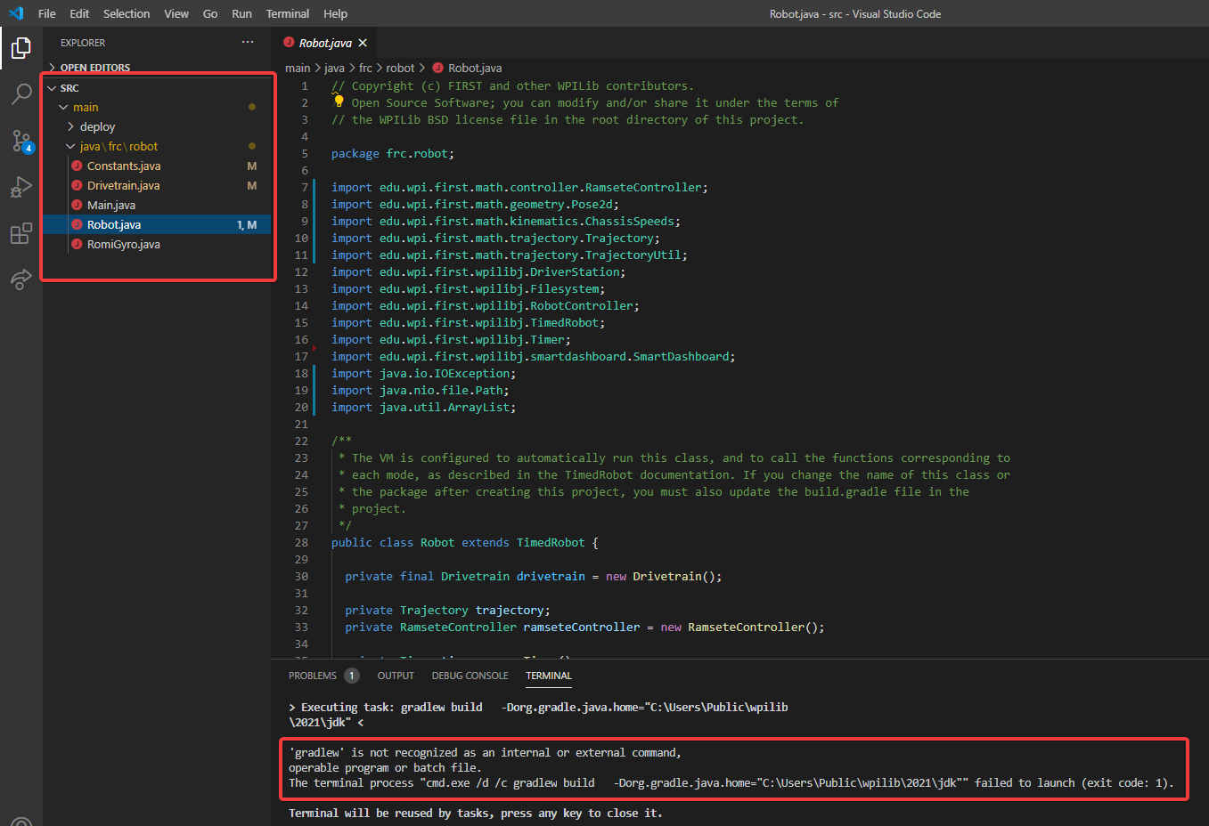
In the above screenshot, you can see that the left-hand sidebar does not contain many files. At a minimum, VS Code needs a couple of files to properly build and deploy your project.
gradlewbuild.gradlegradlew.bat
If you do not see any one of the above files in your project directory, then you have two possible causes.
A corrupt or bad project.
You are in the wrong directory.
Fixing gradlew is not recognized…
gradlew is not recognized... is a fairly easy problem to fix. First identify the problem source:
Are you in the wrong directory? - Verify that the project directory is the correct directory and open this.
Is your project missing essential files? - This issue is more complex to solve. The recommended solution is to recreate your project and manually copy necessary code in.
Support Resources
In addition to the documentation here, there are a variety of other resources available to FRC® teams to help understand the Control System and software.
Other Documentation
In addition to this site there are a few other places teams may check for documentation:
Forums
Stuck? Have a question not answered by the documentation? Official Support is provided on these forums:
NI FRC Community Discussion Section (roboRIO, LabVIEW and Driver Station software questions)
FIRST Inspires Control System Forum (wiring, hardware and Driver Station questions)
FIRST Inspires Programming Forum (programming questions for C++, Java, or LabVIEW)
CTRE Support
Support for Cross The Road Electronics components (Pneumatics Control Module, Power Distribution Panel, Talon SRX, and Voltage Regulator Module) is provided via the email address support@crosstheroadelectronics.com
REV Robotics Support
Support for REV Robotics components (SPARK MAX, Sensors, upcoming new control system components) is provided via phone at 844-255-2267 or via the email address support@revrobotics.com
Other Vendors
Support for vendors outside of the KOP can be found below.
Unofficial Support
There are useful forms of support provided by the community through various forums and services. The below links and websites are not endorsed by FIRST® and are use at your own risk.
Bug Reporting
Found a bug? Let us know by reporting it in the Issues section of the appropriate WPILibSuite project on Github: https://github.com/wpilibsuite
FRC Glossary
- accelerometer
A common sensor used to measure acceleration in one or more axis.
- alliance
A cooperative of up to four (4) FIRST® Robotics Competition teams.
- auto
The first phase of each match is called Autonomous (auto) and consists of the first fifteen (0:15) seconds.
- COTS
Commercial off the shelf, a standard (i.e. not custom order) part commonly available from a vendor to all teams for purchase.
- C++
One of the three officially supported programming languages.
- deprecated
Software that will be maintained for at least 1 year, but may be removed after that.
- DHCP
Dynamic Host Configuration Protocol, the protocol that allows a central device to assign unique IP addresses to all other devices.
- FMS
Field Management System, the electronics core responsible for sensing and controlling the FIRST Robotics Competition field.
- GradleRIO
The mechanism that powers the deployment of robot code to the roboRIO.
- gyroscope
A device that measures rate of rotation. It can add up the rotation measurements to determine heading of the robot. (“gyro”, for short)
- heading
The direction the robot is pointed, usually expressed as an angle in degrees.
- IMU
Inertial Measurement Unit, a sensor that combines both an accelerometer and a gyroscope into a single sensor.
- Java
One of the three officially supported programming languages.
- KOP
Kit of Parts, the collection of items listed on the Kickoff Kit checklists, distributed to the team via FIRST Choice, or paid for completely (except shipping) with a Product Donation Voucher (PDV).
- KOP chassis
The AM14U4 chassis distributed to every team (that did not opt out) as part of the KOP.
- LabVIEW
One of the three officially supported programming languages.
- match
A two (2) minute and thirty (30) second period of time in which an alliance plays a FRC game.
- NetworkTables
A way to communicate key / value pairs, of data, between programs.
- RP
Ranking Point, a way of ordering teams rewarding specific objectives in addition to winning the match.
- simulation
A way for teams to test their code without having an actual robot available.
- teleop
The second phase of each match is called the Teleoperated Period (teleop) and consists of drivers controlling their robots.
- trajectory
A trajectory is a smooth curve, with velocities and accelerations at each point along the curve, connecting two endpoints on the field.
Driver Station
FRC Driver Station Powered by NI LabVIEW
This article describes the use and features of the FRC® Driver Station Powered by NI LabVIEW.
For information on installing the Driver Station software see this document.
Starting the FRC Driver Station
The FRC Driver Station can be launched by double-clicking the icon on the Desktop or by selecting Start->All Programs->FRC Driver Station.
Note
By default the FRC Driver Station launches the LabVIEW Dashboard. It can also be configured on Setup Tab to launch the other Dashboards: SmartDashboard and Shuffleboard.
Setting Up the Driver Station
The DS should be set to your team number in order to connect to your robot. In order to do this click the Setup tab then enter your team number in the team number box. Press return or click outside the box for the setting to take effect.
PCs will typically have the correct network settings for the DS to connect to the robot already, but if not, make sure your Network adapter is set to DHCP.
Status Pane
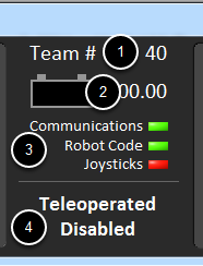
The Status Pane of the Driver Station is located in the center of the display and is always visible regardless of the tab selected. It displays a selection of critical information about the state of the DS and robot:
Team # - The Team number the DS is currently configured for. This should match your FRC team number. To change the team number see the Setup Tab.
Battery Voltage - If the DS is connected and communicating with the roboRIO this displays current battery voltage as a number and with a small chart of voltage over time in the battery icon. The background of the numeric indicator will turn red when the roboRIO brownout is triggered. See roboRIO Brownout and Understanding Current Draw for more information.
Major Status Indicators - These three indicators display major status items for the DS. The “Communications” indicates whether the DS is currently communicating with the FRC Network Communications Task on the roboRIO (it is split in half for the TCP and UDP communication). The “Robot Code” indicator shows whether the team Robot Code is currently running (determined by whether or not the Driver Station Task in the robot code is updating the battery voltage), The “Joysticks” indicator shows if at least one joystick is plugged in and recognized by the DS.
Status String - The Status String provides an overall status message indicating the state of the robot, some examples are “No Robot Communication”, “No Robot Code”, “Emergency Stopped”, and “Teleoperated Enabled”. When the roboRIO brownout is triggered this will display “Voltage Brownout”.
Operation Tab
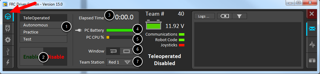
The Operations Tab is used to control the mode of the robot and provide additional key status indicators while the robot is running.
Robot Mode - This section controls the Robot Mode. Practice Mode causes the robot to cycle through the same transitions as an FRC match after the Enable button is pressed (timing for practice mode can be found on the setup tab).
Enable/Disable - These controls enable and disable the robot. See also Driver Station Key Shortcuts
Elapsed Time - Indicates the amount of time the robot has been enabled
PC Battery - Indicates current state of DS PC battery and whether the PC is plugged in
PC CPU% - Indicates the CPU Utilization of the DS PC
Window Mode - When not on the Driver account on the Classmate allows the user to toggle between floating (arrow) and docked (rectangle)
Team Station - When not connected to FMS, sets the team station to transmit to the robot.
Note
When connected to the Field Management System the controls in sections 1, and 2 will be replaced by the words FMS Connected and the control in Section 7 will be greyed out.
Diagnostics Tab
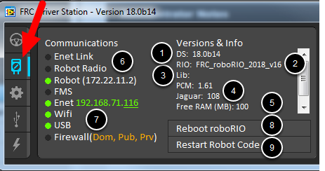
The Diagnostics Tab contains additional status indicators that teams can use to diagnose issues with their robot:
DS Version - Indicates the Driver Station Version number
roboRIO Image Version - String indicating the version of the roboRIO Image
WPILib Version - String indicating the version of WPILib in use
CAN Device Versions - String indicating the firmware version of devices connected to the CAN bus. These items may not be present if the CTRE Phoenix Framework has not been loaded
Memory Stats - This section shows stats about the roboRIO memory
Connection Indicators - The top half of these indicators show connection status to various components.
“Enet Link” indicates the computer has something connected to the ethernet port.
“Robot Radio” indicates the ping status to the robot wireless bridge at 10.XX.YY.1.
“Robot” indicates the ping status to the roboRIO using mDNS (with a fallback of a static 10.TE.AM.2 address).
“FMS” indicates if the DS is receiving packets from FMS (this is NOT a ping indicator).
Network Indicators - The second section of indicators indicates status of network adapters and firewalls. These are provided for informational purposes, communication may be established with one or more unlit indicators in this section
“Enet” indicates the IP address of the detected Ethernet adapter
“WiFi” indicates if a wireless adapter has been detected as enabled
“USB” indicates if a roboRIO USB connection has been detected
“Firewall” indicates if any firewalls are detected as enabled. Enabled firewalls will show in orange ( Dom = Domain, Pub = Public, Prv = Private)
Reboot roboRIO - This button attempts to perform a remote reboot of the roboRIO (after clicking through a confirmation dialog)
Restart Robot Code - This button attempts to restart the code running on the robot (but not restart the OS)
Setup Tab
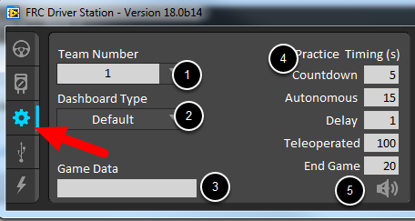
The Setup Tab contains a number of buttons teams can use to control the operation of the Driver Station:
Team Number - Should contain your FRC Team Number. This controls the mDNS name that the DS expects the robot to be at. Shift clicking on the dropdown arrow will show all roboRIO names detected on the network for troubleshooting purposes.
Dashboard Type - Controls what Dashboard is launched by the Driver Station. Default launches the file pointed to by the “FRC DS Data Storage.ini” (for more information about setting a custom dashboard ), by default this is Dashboard.exe in the Program Files (x86)\FRC Dashboard folder. LabVIEW attempts to launch a dashboard at the default location for a custom built LabVIEW dashboard, but will fall back to the default if no dashboard is found. SmartDashboard and Shuffleboard launch the respective dashboards included with the C++ and Java WPILib installation. Remote launches another dashboard from the “DashboardRemoteIP” field in the “FRC DS Data Storage.ini” file.
Game Data - This box can be used for at home testing of the Game Data API. Text entered into this box will appear in the Game Data API on the Robot Side. When connected to FMS, this data will be populated by the field automatically.
Practice Mode Timing - These boxes control the timing of each portion of the practice mode sequence. When the robot is enabled in practice mode the DS automatically proceeds through the modes indicated from top to bottom.
Audio Control - This button controls whether audio tones are sounded when the Practice Mode is used.
USB Devices Tab
The USB Devices tab includes the information about the USB Devices connected to the DS
USB Setup List - This contains a list of all compatible USB devices connected to the DS. Pressing a button on a device will highlight the name in green and put 2 *s before the device name
Rescan - This button will force a Rescan of the USB devices. While the robot is disabled, the DS will automatically scan for new devices and add them to the list. To force a complete re-scan or to re-scan while the robot is Enabled (such as when connected to FMS during a match) press F1 or use this button.
Device indicators - These indicators show the current status of the Axes, buttons and POV of the joystick.
Rumble - For XInput devices (such as X-Box controllers) the Rumble control will appear. This can be used to test the rumble functionality of the device. The top bar is “Right Rumble” and the bottom bar is “Left Rumble”. Clicking and holding anywhere along the bar will activate the rumble proportionally (left is no rumble = 0, right is full rumble = 1). This is a control only and will not indicate the Rumble value set in robot code.
Re-Arranging and Locking Devices
The Driver Station has the capability of “locking” a USB device into a specific slot. This is done automatically if the device is dragged to a new position and can also be triggered by double clicking on the device. “Locked” devices will show up with an underline under the device. A locked device will reserve it’s slot even when the device is not connected to the computer (shown as grayed out and underlined). Devices can be unlocked (and unconnected devices removed) by double clicking on the entry.
Note
If you have two or more of the same device, they should maintain their position as long as all devices remain plugged into the computer in the same ports they were locked in. If you switch the ports of two identical devices the lock should follow the port, not the device. If you re-arrange the ports (take one device and plug it into a new port instead of swapping) the behavior is not determinate (the devices may swap slots). If you unplug one or more of the set of devices, the positions of the others may move, they should return to the proper locked slots when all devices are reconnected.
Example: The image above shows 4 devices:
A Locked “Logitech Attack 3” joystick. This device will stay in this position unless dragged somewhere else or unlocked
An unlocked “Logitech Extreme 3D” joystick
An unlocked “Gamepad F310 (Controller)” which is a Logitech F310 gamepad
A Locked, but disconnected “MadCatz GamePad (Controller)” which is a MadCatz Xbox 360 Controller
In this example, unplugging the Logitech Extreme 3D joystick will result in the F310 Gamepad moving up to slot 1. Plugging in the MadCatz Gamepad (even if the devices in Slots 1 and 2 are removed and those slots are empty) will result in it occupying Slot 3.
CAN/Power Tab
The last tab on the left side of the DS is the CAN/Robot Power Tab. This tab contains information about the power status of the roboRIO and the status of the CAN bus:
Comms Faults - Indicates the number of Comms faults that have occurred since the DS has been connected
12V Faults - Indicates the number of input power faults (Brownouts) that have occurred since the DS has been connected
6V/5V/3.3V Faults - Indicates the number of faults (typically cause by short circuits) that have occurred on the User Voltage Rails since the DS has been connected
CAN Bus Utilization - Indicates the percentage utilization of the CAN bus
CAN faults - Indicates the counts of each of the 4 types of CAN faults since the DS has been connected
If a fault is detected, the indicator for this tab (shown in blue in the image above) will turn red.
Messages Tab
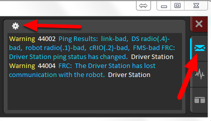
The Messages tab displays diagnostic messages from the DS, WPILib, User Code, and/or the roboRIO. The messages are filtered by severity. By default, only Errors are displayed.
To access settings for the Messages tab, click the Gear icon. This will display a menu that will allow you to select the detail level (Errors, Errors+Warnings or Errors+Warnings+Prints), Clear the box, launch a larger Console window for viewing messages, or launch the DS Log Viewer.
Charts Tab
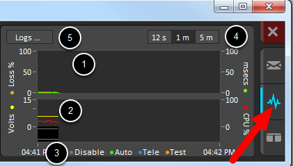
The Charts tab plots and displays advanced indicators of robot status to help teams diagnose robot issues:
The top graph charts trip time in milliseconds in green (against the axis on the right) and lost packets per second in orange (against the axis on the left)
The bottom graph plots battery voltage in yellow (against the axis on the left), roboRIO CPU in red (against the axis on the right), DS Requested mode as a continuous line on the bottom of the chart and robot mode as a discontinuous line above it.
This key shows the colors used for the DS Requested and Robot Reported modes in the bottom chart.
Chart scale - These controls change the time scale of the DS Charts
This button launches the DS Log File Viewer
The DS Requested mode is the mode that the Driver Station is commanding the robot to be in. The Robot Reported mode is what code is actually running based on reporting methods contained in the coding frameworks for each language.
Both Tab
The last tab on the right side is the Both tab which displays Messages and Charts side by side
Driver Station Key Shortcuts
F1 - Force a Joystick refresh.
[ + ] + \ - Enable the robot (the 3 keys above Enter on most keyboards)
Enter - Disable the Robot
Space - Emergency Stop the robot. After an emergency stop is triggered the roboRIO will need to be rebooted before the robot can be enabled again.
Note
Space bar will E-Stop the robot regardless of if the Driver Station window has focus or not
Warning
When connected to FMS in a match, teams must press the Team Station E-Stop button to emergency stop their robot as the DS enable/disable and E-Stop key shortcuts are ignored.
Driver Station Best Practices
This document was created by Steve Peterson, with contributions from Juan Chong, James Cole-Henry, Rick Kosbab, Greg McKaskle, Chris Picone, Chris Roadfeldt, Joe Ross, and Ryan Sjostrand. The original post and follow-up posts can be found here
Want to ensure the driver station isn’t a stopper for your team at the FIRST Robotics Competition (FRC) field? Building and configuring a solid driver station laptop is an easy project for the time between stop build day and your competition. Read on to find lessons learned by many teams over thousands of matches.
Prior To Departing For The Competition
Dedicate a laptop to be used solely as a driver station. Many teams do. A dedicated machine allows you manage the configuration for one goal – being ready to compete at the field. Dedicated means no other software except the FRC-provided Driver Station software and associated Dashboard installed or running.
Use a business-class laptop for your driver station. Why? They’re much more durable than the $300 Black Friday special at Best Buy. They’ll survive being banged around at the competition. Business-class laptops have higher quality device drivers, and the drivers are maintained for a longer period than consumer laptops. This makes your investment last longer. Lenovo ThinkPad T series and Dell Latitude are two popular business-class brands you’ll commonly see at competitions. There are thousands for sale every day on eBay. The laptop provided in recent rookie kits is a good entry level machine. Teams often graduate from it to bigger displays as they do more with vision and dashboards.
Consider used laptops rather than new. The FRC® Driver Station and dashboard software uses very few system resources, so you don’t need to buy a new laptop – instead, buy a cheap 4-5 year old used one. You might even get one donated by a used computer store in your area.
Laptop recommended features
RAM – 4GB of RAM
A display size of 13” or greater, with minimum resolution of 1440x1050.
Ports
A built-in Ethernet port is highly preferred. Ensure that it’s a full-sized port. The hinged Ethernet ports don’t hold up to repeated use.
Use an Ethernet port saver to make your Ethernet connection. This extends the life of the port on the laptop. This is particularly important if you have a consumer-grade laptop with a hinged Ethernet port.
If the Ethernet port on your laptop is dodgy, either replace the laptop (recommended) or buy a USB Ethernet dongle from a reputable brand. Many teams find that USB Ethernet is less reliable than built-in Ethernet, primarily due to cheap hardware and bad drivers. The dongles given to rookies in the KOP have a reputation for working well.
2 USB ports minimum
A keyboard. It’s hard to quickly do troubleshooting on touch-only computers at the field.
A solid-state disk (SSD). If the laptop has a rotating disk, spend $50 and replace it with a SSD.
Updated to the current release of Windows 10 or 11. Being the most common OS now seen at competitions, bugs are more likely to be found and fixed for Windows 10 and 11 than on older Windows versions.
Install all Windows updates a week before the competition. This allows you time to ensure the updates will not interfere with driver station functions. To do so, open the Windows Update settings page and see that you’re up-to-date. Install pending updates if not. Reboot and check again to make sure you’re up to date.
Change “Active Hours” for Windows Updates to prevent updates from installing during competition hours. Navigate to Start -> Settings -> Update & Security -> Windows Update, then select Change active hours. If you’re traveling to a competition, take time zone differences into account. This will help ensure your driver station does not reboot or fail due to update installing on the field.
Remove any 3rd party antivirus or antimalware software. Instead, use Windows Defender on Windows 10 or 11. Since you’re only connecting to the internet for Windows and FRC software updating, the risk is low. Only install software on your driver station that’s needed for driving. Your goal here is to eliminate variables that might interfere with proper operation. Remove any unneeded preinstalled software (“bloatware”) that came with the machine. Don’t use the laptop as your Steam machine for gaming back at the hotel the night before the event. Many teams go as far as having a separate programming laptop.
Avoid managed Windows 10 or 11 installations from the school’s IT department. These deployments are built for the school environment and often come with unwanted software that interferes with your robot’s operation.
Laptop battery / power
Turn off Put the computer to sleep in your power plan for both battery and powered operation.
Turn off USB Selective Suspend:
Right click on the battery/charging icon in the tray, then select Power Options.
Edit the plan settings of your power plan.
Click the Change advanced power settings link.
Scroll down in the advanced settings and disable the USB selective suspend setting for both Battery and Plugged in.
Ensure the laptop battery can hold a charge for at least an hour after making the changes above. This allows plenty of time for the robot and drive team to go through the queue and reach the alliance station without mains power.
Bring a trusted USB and Ethernet cable for use connecting to the roboRIO.
Add retention/strain relief to prevent your joystick/gamepad controllers from falling on the floor and/or yanking on the USB ports. This helps prevent issues with intermittent controller connections.
The Windows user account you use to drive must be a member of the Administrator group.
At The Competition
Turn off Windows firewall using these instructions.
Turn off the Wi-Fi adapter, either using the dedicated hardware Wi-Fi switch or by disabling it in the Adapter Settings control panel.
Charge the driver station when it’s in the pit.
Remove login passwords or ensure everyone on the drive team knows the password. You’d be surprised at how often drivers arrive at the field without knowing the password for the laptop.
Ensure your LabView code is deployed permanently and set to “run as startup”, using the instructions in the LabView Tutorial. If you must deploy code every time you turn the robot on, you’re doing it wrong.
Limit web browsing to FRC related web sites. This minimizes the chance of getting malware during the competition.
Don’t plan on using internet access to do software updates. There likely won’t be any in the venue, and hotel Wi-Fi varies widely in quality. If you do need updates, contact a Control System Advisor in the pit.
Before Each Match
Make sure the laptop is on and logged in prior to the end of the match before yours.
Close programs that aren’t needed during the match – e.g., Visual Studio Code or LabView – when you are competing.
Bring your laptop charger to the field. Power is provided for you in each player station.
Fasten your laptop with hook-and-loop tape to the player station shelf. You never know when your alliance partner will have an autonomous programming issue and blast the wall.
Ensure joysticks and controllers are assigned to the correct USB ports.
In the USB tab in the FRC Driver Station software, drag and drop to assign joysticks as needed.
Use the rescan button (F1) if joysticks / controllers do not appear green
Use the rescan button (F1) during competition if joystick or controllers become unplugged and then are plugged back in or otherwise turn gray during competition.
Driver Station Log File Viewer
In an effort to provide information to aid in debugging, the FRC® Driver Station creates log files of important diagnostic data while running. These logs can be reviewed later using the FRC Driver Station Log Viewer. The Log Viewer can be found via the shortcut installed in the Start menu or in the FRC Driver Station folder in Program Files.
Event Logs
The Driver Station logs all messages sent to the Messages box on the Diagnostics tab (not the User Messages box on the Operation tab) into a new Event Log file. When viewing Log Files with the Driver Station Log File Viewer, the Event Log and DSLog files are overlaid in a single display.
Log Viewer UI
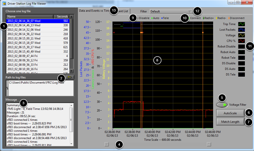
The Log Viewer contains a number of controls and displays to aid in the analysis of the Driver Station log files:
File Selection Box - This window displays all available log files in the currently selected folder. Click on a log file in the list to select it.
Path to Log Files - This box displays the current folder the viewer is looking in for log files. This defaults to the folder that the Driver Station stores log files in. Click the folder icon to browse to a different location.
Message Box - This box displays a summary of all messages from the Event Log. When hovering over an event on the graph this box changes to display the information for that event.
Scroll Bar - When the graph is zoomed in, this scroll bar allows for horizontal scrolling of the graph.
Voltage Filter - This control turns the Voltage Filter on and off (defaults to on). The Voltage Filter filters out data such as CPU %, robot mode and trip time when no Battery Voltage is received (indicating that the DS is no in communication with the roboRIO).
AutoScale - This button zooms the graph out to show all data in the log.
Match Length - This button scales the graph to approximately the length of an FRC match (2 minutes and 30 seconds shown). It does not automatically locate the start of the match, you will have to scroll using the scroll bar to locate the beginning of the Autonomous mode.
Graph - This display shows graph data from the DS Log file (voltage, trip time, roboRIO CPU%, Lost Packets, and robot mode) as well as overlaid event data (shown as dots on the graph with select events showing as vertical lines across the entire graph). Hovering over event markers on the graph displays information about the event in the Messages window in the bottom left of the screen.
Robot Mode Key - Key for the Robot Mode displayed at the top of the screen
Major event key - Key for the major events, displayed as vertical lines on the graph
Graph key - Key for the graph data
Filter Control - Drop-down to select the filter mode (filter modes explained below)
Tab Control - Control to switch between the Graph (Data and Events vs. Time) and Event List displays.
Using the Graph Display
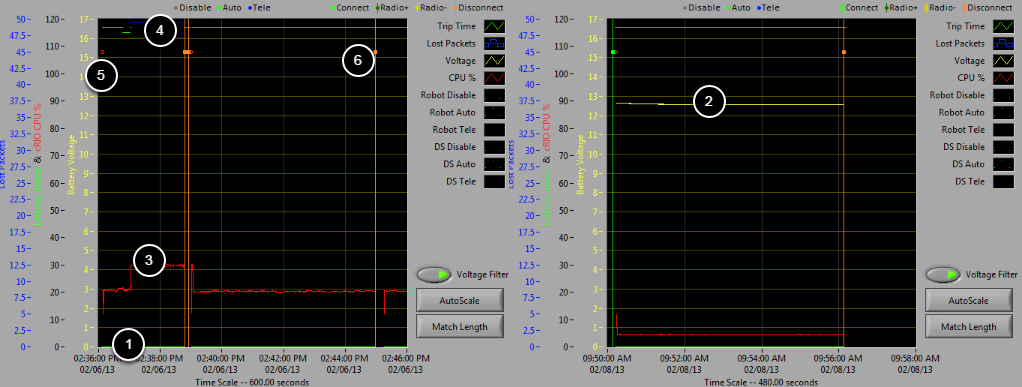
The Graph Display contains the following information:
Graphs of Trip Time in ms (green line) and Lost Packets per second (displayed as blue vertical bars). In these example images Trip Time is a flat green line at the bottom of the graph and there are no lost packets
Graph of Battery voltage displayed as a yellow line.
Graph of roboRIO CPU % as a red line
Graph of robot mode and DS mode. The top set of the display shows the mode commanded by the Driver Station. The bottom set shows the mode reported by the robot code. In this example the robot is not reporting it’s mode during the disabled and autonomous modes, but is reported during Teleop.
Event markers will be displayed on the graph indicating the time the event occurred. Errors will display in red; warnings will display in yellow. Hovering over an event marker will display information about the event in the Messages box at the bottom left of the screen.
Major events are shown as vertical lines across the graph display.
To zoom in on a portion of the graph, click and drag around the desired viewing area. You can only zoom the time axis, you cannot zoom vertically.
Event List
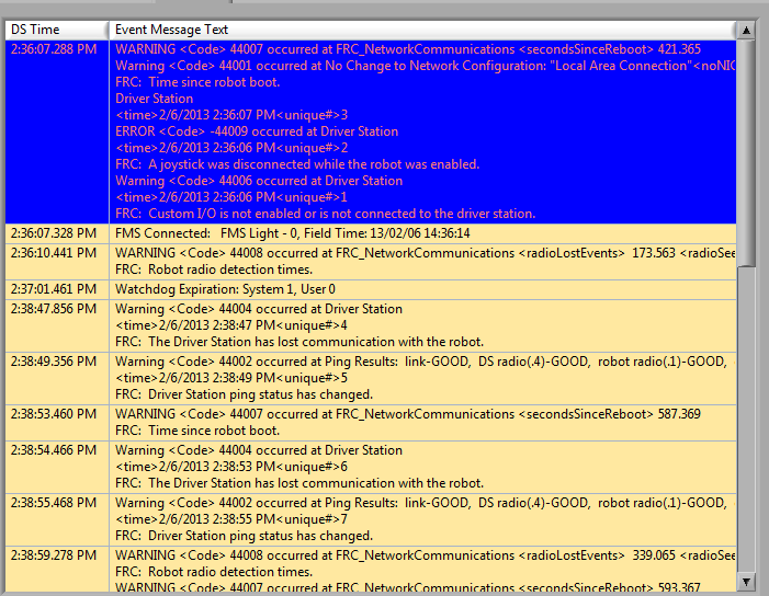
The Event List tab displays a list of events (warnings and errors) recorded by the Driver Station. The events and detail displayed are determined by the currently active filter (images shows “All Events, All Info” filter active).
Filters
Three filters are currently available in the Log Viewer:
Default: This filter filters out many of the errors and warnings produced by the Driver Station. This filter is useful for identifying errors thrown by the code on the Robot.
All Events and Time: This filter shows all events and the time they occurred
All Events, All Info: This filter shows all events and all recorded info. At this time the primary difference between this filter and “All Events and Time” is that this option shows the “unique” designator for the first occurrence of a particular message.
Identifying Logs from Matches

A common task when working with the Driver Station Logs is to identify which logs came from competition matches. Logs which were taken during a match can now be identified using the FMS Connected event which will display the match type (Practice, Qualification or Elimination), match number, and the current time according to the FMS server. In this example, you can see that the FMS server time and the time of the Driver Station computer are fairly close, approximately 7 seconds apart.
Identifying Common Connection Failures with the Log Viewer
When diagnosing robot issues, there is no substitute for thorough knowledge of the system and a methodical debugging approach. If you need assistance diagnosing a connection problem at your events it is strongly recommended to seek assistance from your FTA and/or CSA. The goal of this section is to familiarize teams with how some common failures can manifest themselves in the DS Log files. Please note that depending on a variety of conditions a particular failure show slightly differently in a log file.
Note
Note that all log files shown in this section have been scaled to match length using the Match Length button and then scrolling to the beginning of the autonomous mode. Also, many of the logs do not contain battery voltage information, the platform used for log capture was not properly wired for reporting the battery voltage.
Tip
Some error messages that are found in the Log Viewer are show below and more are detailed in the Driver Station Errors/Warnings article.
“Normal” Log
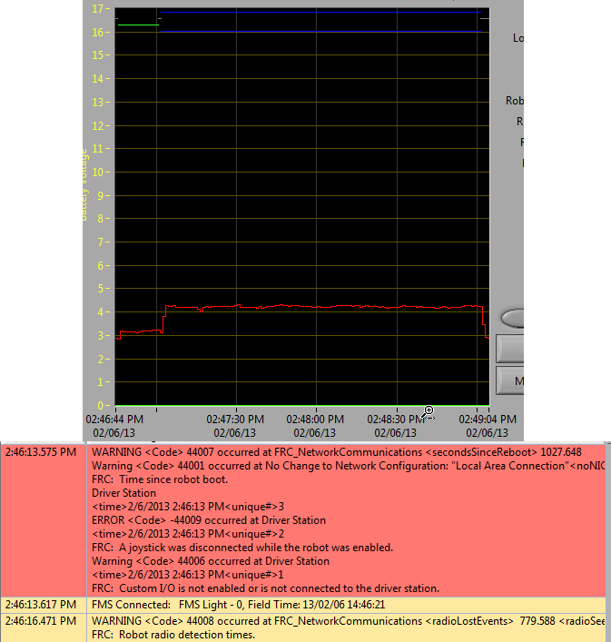
This is an example of a normal match log. The errors and warnings contained in the first box are from when the DS first started and can be ignored. This is confirmed by observing that these events occurred prior to the “FMS Connected:” event. The last event shown can also be ignored, it is also from the robot first connecting to the DS (it occurs 3 seconds after connecting to FMS) and occurs roughly 30 seconds before the match started.
Disconnected from FMS
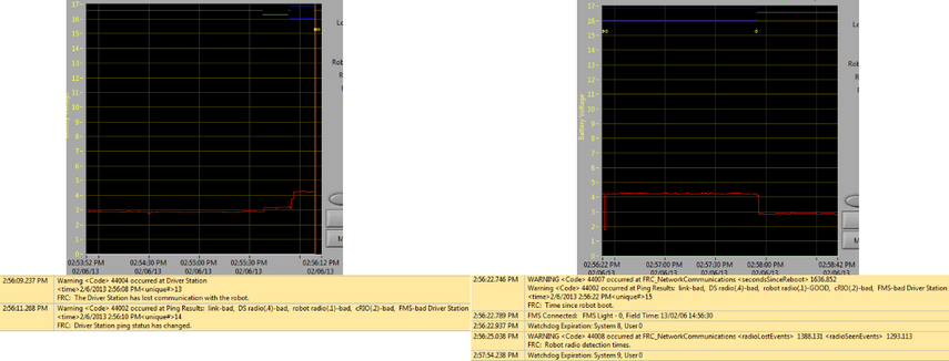
When the DS disconnects from FMS, and therefore the robot, during the match it may segment the log into pieces. The key indicators to this failure are the last event of the first log, indicating that the connection to FMS is now “bad” and the second event from the 2nd log which is a new FMS connected message followed by the DS immediately transitioning into Teleop Enabled. The most common cause of this type of failure is an ethernet cable with no latching tab or a damaged ethernet port on the DS computer.
roboRIO Reboot
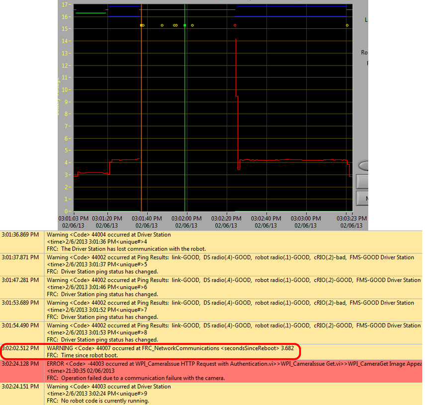
The “Time since robot boot” message is the primary indicator in a connection failure caused by the roboRIO rebooting. In this log the DS loses connection with the roboRIO at 3:01:36 as indicated by the first event. The second event indicates that the ping initiated after the connection failed was successful to all devices other than the roboRIO. At 3:01:47 the roboRIO begins responding to pings again, one additional ping fails at 3:01:52. At 3:02:02 the Driver Station connects to the roboRIO and the roboRIO reports that it has been up for 3.682 seconds. This is a clear indicator that the roboRIO has rebooted. The code continues to load and at 3:02:24 the code reports an error communicating with the camera. A warning is also reported indicating that no robot code is running right before the code finishes starting up.
Ethernet cable issue on robot
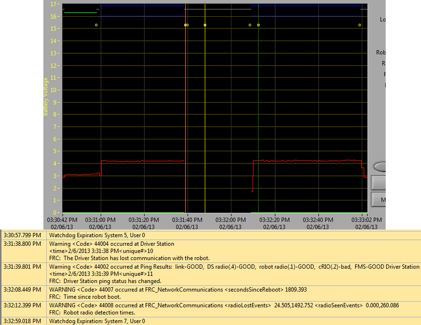
An issue with the ethernet cable on the robot is primarily indicated by the ping to the roboRIO going to bad and Radio Lost and Radio Seen events when the roboRIO reconnects. The “Time since robot boot” message when the roboRIO reconnects will also indicate that the roboRIO has not rebooted. In this example, the robot Ethernet cable was disconnected at 3:31:38. The ping status indicates that the radio is still connected. When the robot reconnects at 3:32:08 the “Tim since robot boot” is 1809 seconds indicating that the roboRIO clearly did not reboot. At 3:32:12 the robot indicates that it lost the radio 24.505 seconds ago and it returned 0.000 seconds ago. These points are plotted as vertical lines on the graph, yellow for radio lost and green for radio seen. Note that the times are slightly offset from the actual events as shown via the disconnection and connection, but help to provide additional information about what is occurring.
Radio reboot
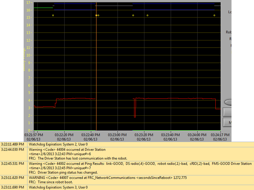
A reboot of the robot radio is typically characterized by a loss of connection to the radio for ~40-45 seconds. In this example, the radio briefly lost power at 3:22:44, causing it to start rebooting. The event at 3:22:45 indicates that the ping to the radio failed. At 3:23:11, the DS regains communication with the roboRIO and the roboRIO indicates it has been up for 1272.775 seconds, ruling out a roboRIO reboot. Note that the network switch on the radio comes back up very quickly so a momentary power loss may not result in a “radio lost”/”radio seen” event pair. A longer disturbance may result in radio events being logged by the DS. In that case, the distinguishing factor which points towards a radio reboot is the ping status of the radio from the DS. If the radio resets, the radio will be unreachable. If the issue is a cabling or connection issue on the robot, the radio ping should remain “GOOD”.
Driver Station Errors/Warnings
In an effort to provide both Teams and Volunteers (FTAs/CSAs/etc.) more information to use when diagnosing robot problems, a number of Warning and Error messages have been added to the Driver Station. These messages are displayed in the DS diagnostics tab when they occur and are also included in the DS Log Files that can be viewed with the Log File Viewer. This document discusses the messages produced by the DS (messages produced by WPILib can also appear in this box and the DS Logs).
Joystick Unplugged
ERROR<Code>-44009 occurred at Driver Station
<time>2/5/2013 4:43:54 PM <unique#>1
FRC: A joystick was disconnected while the robot was enabled.
This error is triggered when a Joystick is unplugged. Contrary to the message text this error will be printed even if the robot is not enabled, or even connected to the DS. You will see a single instance of this message occur each time the Driver Station is started, even if Joysticks are properly connected and functioning.
Lost Communication
Warning<Code>44004 occurred at Driver Station
<time>2/6/2013 11:07:53 AM<unique#>2
FRC: The Driver Station has lost communication with the robot.
This Warning message is printed whenever the Driver Station loses communication with the robot (Communications indicator changing from green to red). A single instance of this message is printed when the DS starts up, before communication is established.
Ping Status
Warning<Code>44002 occurred at Ping Results: link-GOOD, DS radio(.4)-bad, robot radio(.1)-GOOD, cRIO(.2)-bad, FMS- bad Driver Station
<time>2/6/2013 11:07:59 AM<unique#>5
FRC: Driver Station ping status has changed.
A Ping Status warning is generated each time the Ping Status to a device changes while the DS is not in communication with the roboRIO. As communications is being established when the DS starts up, a few of these warnings will appear as the Ethernet link comes up, then the connection to the robot radio, then the roboRIO (with FMS mixed in if applicable). If communications are later lost, the ping status change may help identify at which component the communication chain broke.
Time Since Robot Boot
WARNING<Code>44007 occurred at FRC_NetworkCommunications
**<secondsSinceReboot> 3.585**
FRC: Time since robot boot.
This message is printed each time the DS begins communicating with the roboRIO. The message indicates the up-time, in seconds, of the roboRIO and can be used to determine if a loss of communication was due to a roboRIO Reboot.
Radio Detection Times
WARNING<Code>44008 occurred at FRC_NetworkCommunications
<radioLostEvents> 19.004<radioSeenEvents> 0.000
FRC: Robot radio dectection times
WARNING<Code>44008 occurred at FRC_NetworkCommunications
<radioLostEvents> 2.501,422.008<radioSeenEvents> 0.000,147.005
FRC: Robot radio dectection times.
This message may be printed when the DS begins communicating with the roboRIO and indicates the time, in seconds, since the last time the radio was lost and seen. In the first example image above the message indicates that the roboRIO’s connection to the radio was lost 19 seconds before the message was printed and the radio was seen again right when the message was printed. If multiple radioLost or radioSeen events have occurred since the roboRIO booted, up to 2 events of each type will be included, separated by commas.
No Robot Code
Warning<Code>44003 occurred at Driver Station
<time>2/8/2013 9:50:13 AM<unique#>8
FRC: No robot code is currently running.
This message is printed when the DS begins communicating with the roboRIO, but detects no robot code running. A single instance of this message will be printed if the Driver Station is open and running while the roboRIO is booting as the DS will begin communication with the roboRIO before the robot code finishes loading.
Programming Radios for FMS Offseason
When using the FMS Offseason software, the typical networking setup is to use a single access point with a single SSID and WPA key. This means that the radios should all be programmed to connect to this network, but with different IPs for each team. The Team version of the FRC® Bridge Configuration Utility has an FMS Offseason mode that can be used to do this configuration.
Pre-Requisites
Install the FRC® Radio Configuration Utility software per the instructions in Programming your radio
Before you begin using the software:
Disable WiFi connections on your computer, as it may prevent the configuration utility from properly communicating with the bridge
Plug directly from your computer into the wireless bridge ethernet port closest to the power jack. Make sure no other devices are connected to your computer via ethernet. If powering the radio via PoE, plug an Ethernet cable from the PC into the socket side of the PoE adapter (where the roboRIO would plug in). If you experience issues configuring through the PoE adapter, you may try connecting the PC to the alternate port on the radio.
Programmed Configuration
The Radio Configuration Utility programs a number of configuration settings into the radio when run. These settings apply to the radio in all modes (including at events). These include:
Set a static IP of
10.TE.AM.1Set an alternate IP on the wired side of
192.168.1.1for future programmingBridge the wired ports so they may be used interchangeably
The LED configuration noted in the status light referenced below.
4Mb/s bandwidth limit on the outbound side of the wireless interface (may be disabled for home use)
QoS rules for internal packet prioritization (affects internal buffer and which packets to discard if bandwidth limit is reached). These rules are:
Robot Control and Status (UDP
1110,1115,1150)Robot TCP & NetworkTables (TCP
1735,1740)Bulk (All other traffic). (disabled if BW limit is disabled)
DHCP server enabled. Serves out:
10.TE.AM.11-10.TE.AM.111on the wired side10.TE.AM.138-10.TE.AM.237on the wireless sideSubnet mask of
255.255.255.0Broadcast address
10.TE.AM.255
DNS server enabled. DNS server IP and domain suffix (
.lan) are served as part of the DHCP.
Tip
See the Status Light Reference for details on the behavior of the radio status lights when configured.
When programmed with the team version of the Radio Configuration - Utility, the user accounts will be left at (or set to) the firmware - defaults for the DAPs only:
Username: root
Password: root
Note
It is not recommended to modify the configuration manually
Launch the software
Use the Start menu or desktop shortcut to launch the program.
Note
If you need to locate the program, it is installed to C:\Program Files (x86)\FRC Radio Configuration Utility. For 32-bit machines the path is C:\Program Files\FRC Radio Configuration Utility
Allow the program to make changes, if prompted
A prompt may appear about allowing the configuration utility to make changes to the computer. Click Yes if the prompt appears.
Enter WPA Key
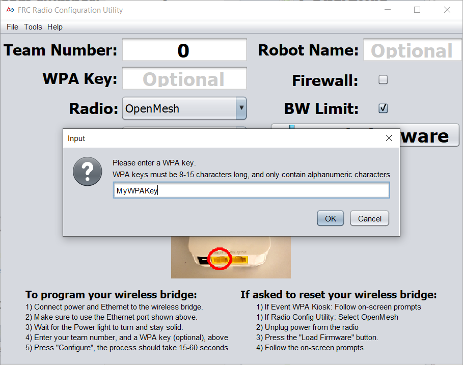
Enter the WPA key for your network in the box and click OK. Leave the box blank if you are using an unsecured network.
Program Radios
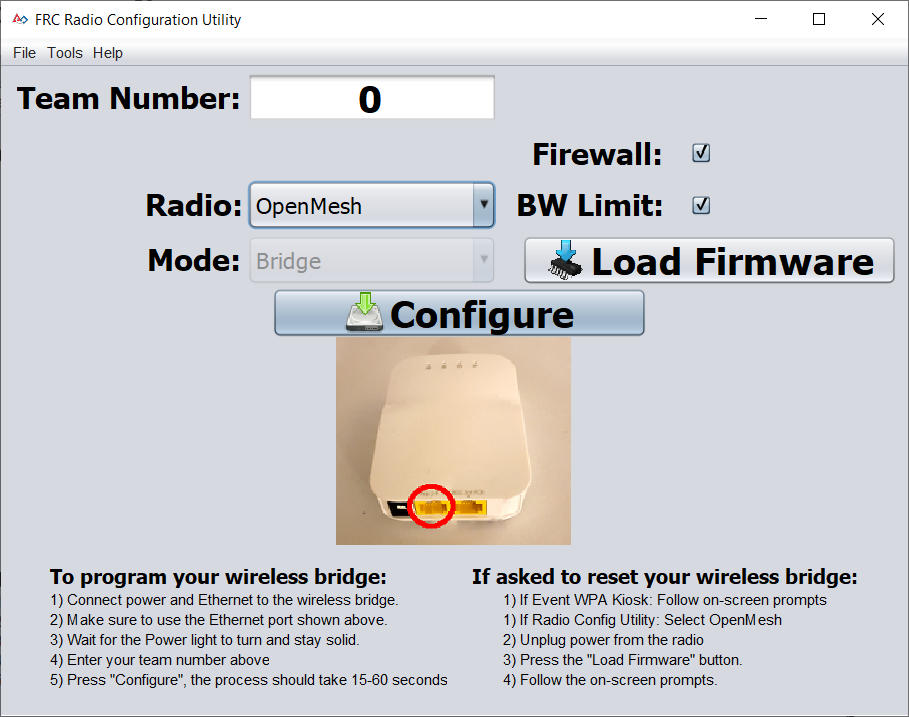
The Kiosk is now ready to program any number of radios to connect to the network entered. To program each radio, connect the radio to the Kiosk, set the Team Number in the box, and click Configure.
The kiosk will program OpenMesh, D-Link Rev A or D-Link Rev B radios to work on an offseason FMS network by selecting the appropriate option from the “Radio” dropdown.
Note
Bandwidth limitations and QoS will not be configured on the D-Link radios in this mode.
Changing SSID or Key
If you enter something incorrectly or need to change the SSID or WPA Key, go to the Tools menu and click FMS-Lite Mode to take the kiosk out of FMS-Lite Mode. When you click again to put the Kiosk back in FMS-Lite Mode, you will be re-prompted for the SSID and Key.
Troubleshooting
See the troubleshooting steps in Programming your radio
Imaging your Classmate (Veteran Image Download)
Note
Veteran teams are not required to re-image their classmate
This document describes the procedure for creating a bootable USB drive to restore the FRC® image on a Classmate computer. If you do not wish to re-image your Classmate then you can start with the appropriate document for C++/Java, LabVIEW, or DS only.
Prerequisites
E09, E11, E12, or E14 Classmate computer or Acer ES1 computer
16GB or larger USB drive
7-Zip software installed (download here). As of the writing of this document, the current released version is 19.00 (2019-02-21).
RMprepUSB software installed (download here). Scroll down the page and select the stable (Full) version download link. As of the writing of this document, the current stable version is 2.1.745.
Download the Computer Image
Download the image from the FIRST FRC Driver Station System Image Portal. There are several computer images available, one for each model. On the download site, select the option that matches your computer by clicking the button below the image. Due to the limited size of the hard drive in the E09, it is supported with a DS/Utilities image only and does not have the IDEs for LabVIEW or C++/Java installed. All other images have the LabVIEW base installation already present.
Note
These images only install the prerequisite core FRC software, it is still necessary to install the FRC specific updates. See the Update Software step for more information.
Warning
Due to computer availability, the E14 image provided is the 2018 image. If using this image, teams may need to remove the old IDE (LabVIEW or Eclipse) and install the new IDE.
Preparation
Place the image file downloaded from the site to a folder on your root drive (e.g.
C:\2016_Image).Connect 16GB or larger USB Flash drive to the PC to use as the new restoration drive.
RMPrep
Start/Run RMprepUSB
Select USB Drive
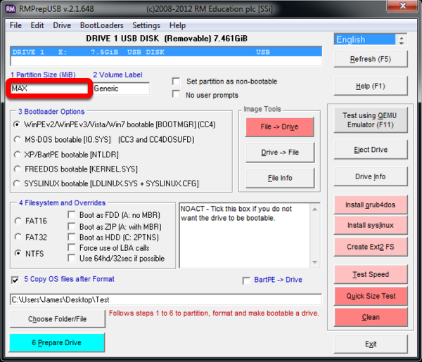
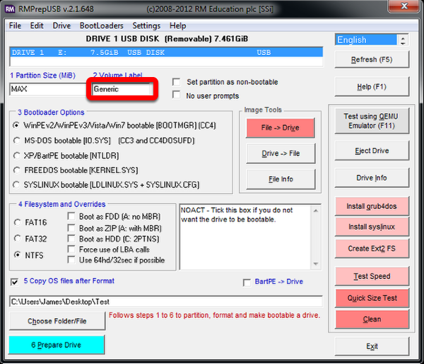
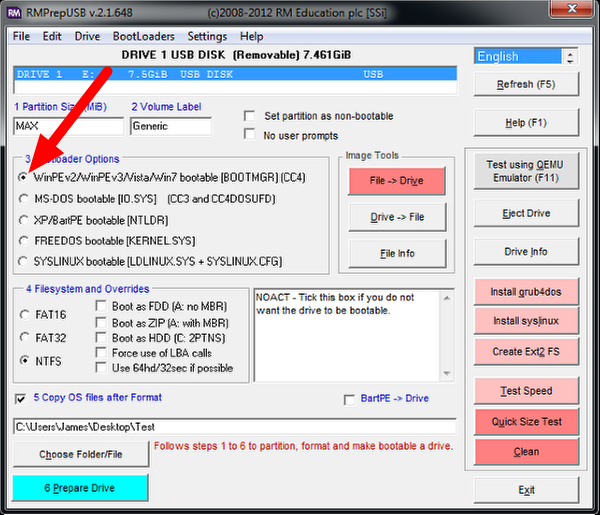

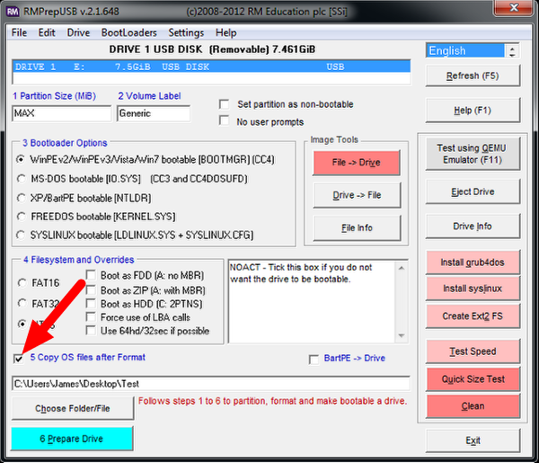
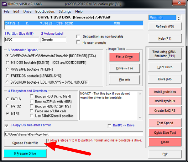
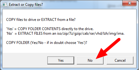
Prepare Drive
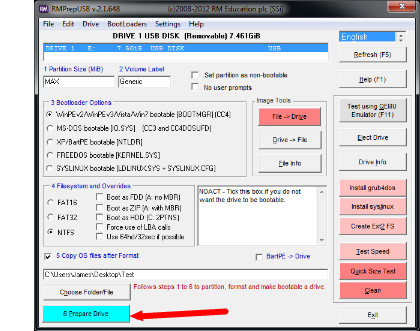
All configuration settings are now complete. Select “Prepare Drive” to begin the process
Confirmation Dialog 1
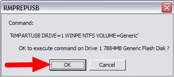
Click “OK” to execute the command on the selected USB Flash drive. A Command Prompt will open showing the progress
Confirmation Dialog 2
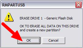
Click “OK” to format the USB drive
Danger
ALL DATA ON THE DRIVE WILL BE ERASED!
Decryption
Note
If you are using an encrypted version of the image downloaded before kickoff you will be prompted to enter the decryption key found at the end of the Kickoff video.
Copy Complete
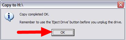
Once formatting is complete, the restoration files will be extracted and copied to the USB drive. This process should take ~15 minutes when connected to a USB 2.0 port. When all files have been copied, this message will appear, press OK to continue.
Eject Drive
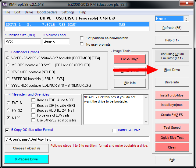
Press the “Eject Drive” button to safely remove the USB drive. The USB drive is now ready to be used to restore the image onto the PC.
Hardware Setup
Make sure the computer is turned off, but plugged in.
Insert the USB Thumb Drive into a USB port on the Driver Station computer.
Boot to USB
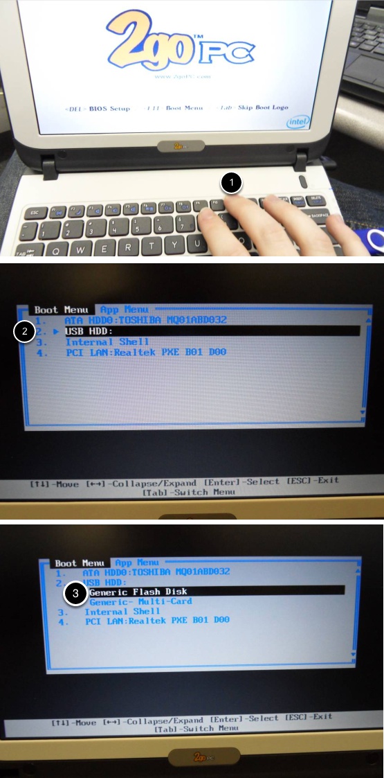
Classmate:
Power on the Classmate and tap the F11 key on the keyboard. Tapping the F11 key during boot will bring up the boot menu.
Use the up/down keys to select the USB HDD: entry on the menu, then press the right arrow to expand the listing
Use the up/down arrow keys on the keyboard to select the USB device (it will be called “Generic Flash Disk”). Press the ENTER key when the USB device is highlighted.
Acer ES1:
Power on the computer and tap the F12 key on the keyboard. Tapping the F12 key during boot will bring up the boot menu.
Use the up/down keys to select the USB HDD: Generic entry on the menu, then press the ENTER key when the USB device is highlighted.
Acer ES1: If pressing F12 does not pull up the boot menu or if the USB device is not listed in the boot menu, see “Checking BIOS Settings” at the bottom of this article.
Image the Classmate
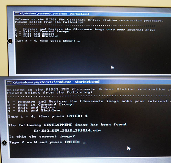
To confirm that you want to reimage the Classmate, type “1” and press ENTER.
Then, type “Y” and press ENTER. The Classmate will begin re-imaging. The installation will take 15-30 minutes.
When the installation is complete, remove the USB drive.
Restart the Classmate. The Classmate will boot into Windows.
Initial Driver Station Boot
The first time the Classmate is turned on, there are some unique steps, listed below, that you’ll need to take. The initial boot may take several minutes; make sure you do not cycle power during the process.
Note
These steps are only required during original startup.
Enter Setup
Log into the Developer account.
Click “Ask me later”.
Click “OK”. The computer now enters a Set Up that may take a few minutes.
Activate Windows
Establish an Internet connection.
Once you have an Internet connection, click the Start menu, right click “Computer” and click “Properties”.
Scroll to the bottom section, “Windows activation”, and Click “Activate Windows now”
Click “Activate Windows online now”. The activation may take a few minutes.
When the activation is complete, close all of the windows.
Microsoft Security Essentials
Navigate through the Microsoft Security Essentials Setup Wizard. Once it is complete, close all of the windows.
Acer ES1: Fix Wireless Driver
Acer ES1 PC only!
The default wireless driver in the image may have issues with intermittent communication with the robot radio. The correct driver is in the image, but could not be set to load by default. To load the correct driver, open the Device Manager by clicking start, typing “Device Manager” in the box and clicking Device Manager.
Open Wireless Device Properties
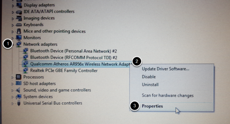
Click on the arrow next to Network Adapters to expand it and locate the Wireless Network Adapter. Right click the adapter and select Properties.
Uninstall-Driver
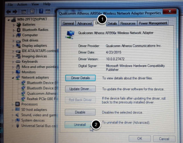
Click on the Driver tab, then click the Uninstall button. Click Yes at any prompts.
Scan for New Hardware
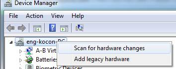
Right click on the top entry of the tree and click “Scan for hardware changes”. The wireless adapter should automatically be re-detected and the correct driver should be installed.
Update Software
In order for the Classmate images to be prepared on time, they are created before the final versions of the software were ready. To use the software for FRC some additional components will need to be installed. LabVIEW teams should continue with Installing the FRC Game Tools (All Languages). C++ or Java teams should continue Installing C++ and Java Development Tools for FRC.
Errors during Imaging Process
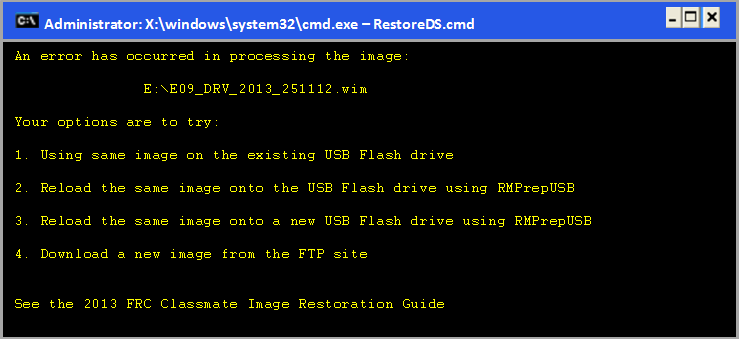
If an error is detected during the imaging process, the following screen will appear. Note that the screenshot below shows the error screen for the Driver Station-only image for the E09. The specific image filename shown will vary depending on the image being applied.
The typical reason for the appearance of this message is due to an error with the USB device on which the image is stored. Each option is listed below with further details as to the actions you can take in pursuing a solution. Pressing any key once this error message is shown will return the user to the menu screen shown in Image the Classmate.
Option 1
- Using same image on the existing USB Flash drive
To try this option, press any key to return to the main menu and select #1. This will run the imaging process again.
Option 2
- Reload the same image onto the USB Flash drive using RMPrepUSB
It’s possible the error message was displayed due to an error caused during the creation of the USB Flash drive (e.g. file copy error, data corruption, etc.) Press any key to return to the main menu and select #4 to safely shutdown the Classmate then follow the steps starting with RMPrep to create a new USB Restoration Key using the same USB Flash drive.
Option 3
- Reload the same image onto a new USB Flash drive using RMPrepUSB
The error message displayed may also be caused by an error with the USB Flash drive itself. Press any key to return to the main menu and select #4 to safely shutdown the Classmate. Select a new USB Flash drive and follow the steps starting with RMPrep.
Option 4
- Download a new image
An issue with the downloaded image may also cause an error when imaging. Press any key to return to the main menu and select #4 to safely shutdown the Classmate. Staring with Download the Classmate Image create a new copy of the imaging stick.
Checking BIOS Settings
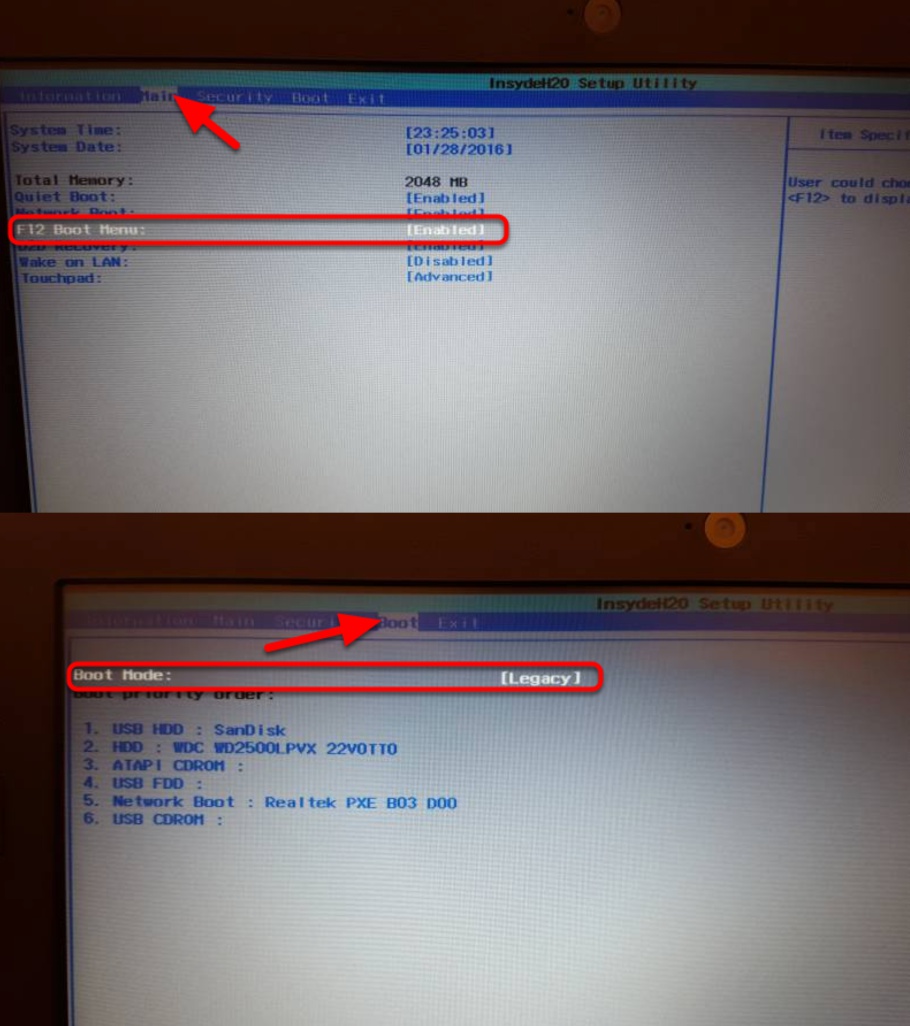
If you are having difficulty booting to USB, check the BIOS settings to insure they are correct. To do this:
Repeatedly tap the F2 key while the computer is booting to enter the BIOS settings
Once the BIOS settings screen has loaded, use the right and left arrow keys to select the “Main” tab, then check if the line for “F12 Boot Menu” is set to “Enabled”. If it is not, use the Up/Down keys to highlight it, press Enter, use Up/Down to select “Enabled” and press Enter again.
Next, use the Left/Right keys to select the “Boot” tab. Make sure that the “Boot Mode” is set to “Legacy”. If it is not, highlight it using UpDown, press Enter, highlight “Legacy” and press Enter again. Press Enter to move through any pop-up dialogs you may see.
Press F10 to save any changes and exit.
Manually Setting the Driver Station to Start Custom Dashboard
Note
If WPILib is not installed to the default location (such as when files are copied to a PC manually), the dashboard of choice may not launch properly. To have the DS start a custom dashboard when it starts up, you have to manually modify the settings for the default dashboard.
Warning
This is not needed for most installations, try using the appropriate Dashboard Type setting for your language first.
Set Driver Station to Default
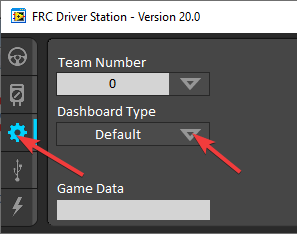
Open the Driver Station software, click on the Setup tab and set the Dashboard setting to Default. Then close the Driver Station!
Locate Dashboard JAR file
Find the location of the dashboard jar file.
Open DS Data Storage file
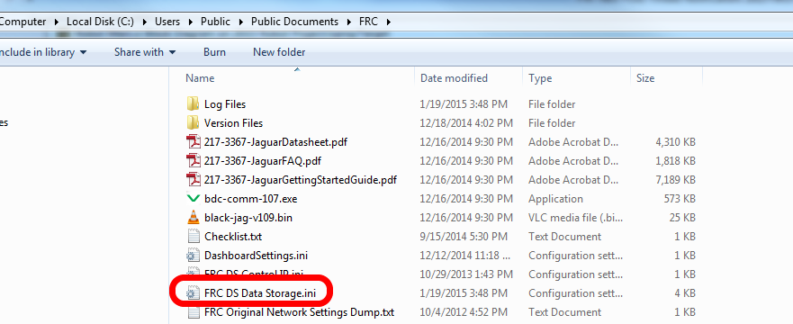
Browse to C:\Users\Public\Documents\FRC and double click on FRC DS Data Storage to open it.
DashboardCmdLine
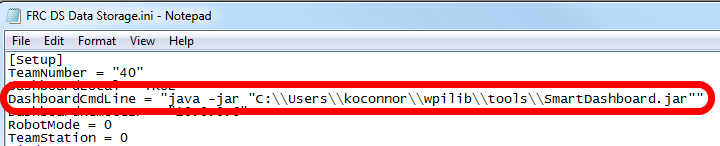
Locate the line beginning with DashboardCmdLine. Modify it to point to the dashboard to launch when the driver station starts
LabVIEW Custom Dashboard
Replace the string after = with "C:\\PATH\\TO\\DASHBOARD.exe" where the path specified is the path to the dashboard exe file. Save the FRC DS Data Storage file.
Java Dashboard
Replace the string after = with java -jar "C:\\PATH\\TO\\DASHBOARD.jar" where the path specified is the path to the dashboard jar file. Save the FRC DS Data Storage file.
Tip
Shuffleboard and Smartdashboard require Java 11.
Dashboard from WPILib installer
Replace the string after = with wscript "C:\\Users\\Public\\wpilib\\YYYY\\tools\\DASHBOARD.vbs" where YYYY is the year and DASHBOARD.vbs is either Shuffleboard.vbs or Smartdashboard.vbs. Save the FRC DS Data Storage file.
Launch Driver Station
The Driver Station should now launch the dashboard each time it is opened.
RobotBuilder
RobotBuilder - Introduction
RobotBuilder Overview
RobotBuilder is an application designed to aid the robot development process. RobotBuilder can help you:
Generating boilerplate code.
Organize your robot and figure out what its key subsystems are.
Check that you have enough channels for all of your sensors and actuators.
Generate wiring diagrams.
Easily modify your operator interface.
More…
Creating a program with RobotBuilder is a very straight forward procedure by following a few steps that are the same for any robot. This lesson describes the steps that you can follow. You can find more details about each of these steps in subsequent sections of the document.
Note
RobotBuilder generates code using the new Command Framework. For more details on the new framework see Command Based Programming.
Divide the Robot into Subsystems
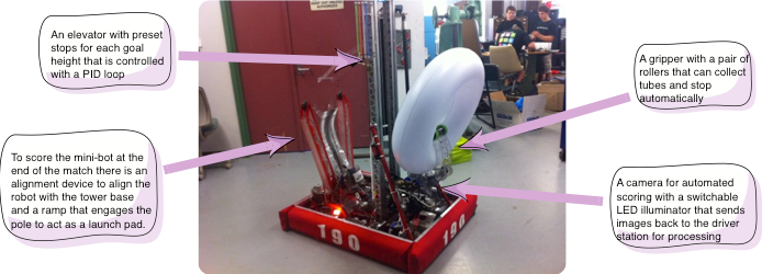
Your robot is naturally made up of a number of smaller systems like the drive trains, arms, shooters, collectors, manipulators, wrist joints, etc. You should look at the design of your robot and break it up into smaller, separately operated subsystems. In this particular example there is an elevator, a minibot alignment device, a gripper, and a camera system. In addition one might include the drive base. Each of these parts of the robot are separately controlled and make good candidates for subsystems.
For more information see Creating a Subsystem.
Adding each Subsystem to the Project
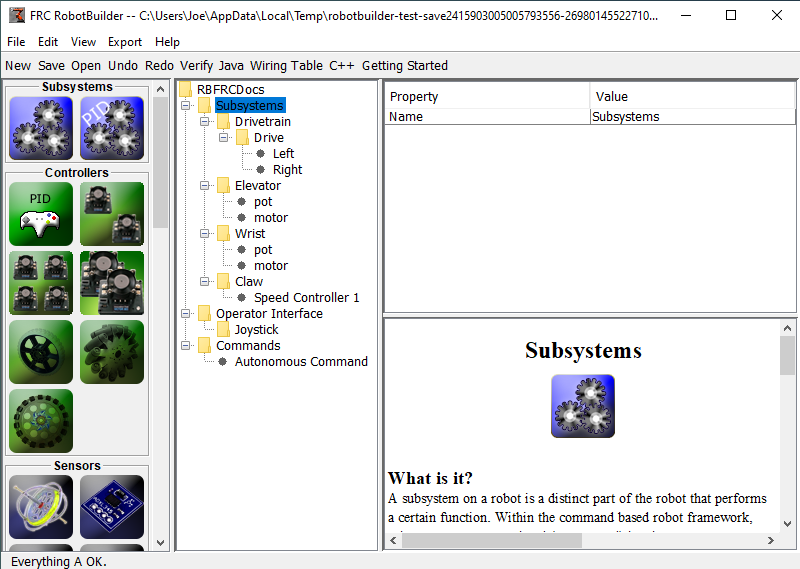
Each subsystem will be added to the “Subsystems” folder in the RobotBuilder and given a meaningful name. For each of the subsystems there are several attributes that get filled in to specify more information about the subsystems. In addition there are two types of subsystems that you might want to create:
PIDSubsystems - often it is desirable to control a subsystems operation with a PID controller. This is code in your program that makes the subsystem element, for example arm angle, more quickly to a desired position then stop when reaching it. PIDSubsystems have the PID Controller code built-in and are often more convenient then adding it yourself. PIDSubsystems have a sensor that determines when the device has reached the target position and an actuator (motor controller) that is driven to the setpoint.
Regular subsystem - these subsystems don’t have an integrated PID controller and are used for subsystems without PID control for feedback or for subsystems requiring more complex control than can be handled with the default embedded PID controller.
As you look through more of this documentation the differences between the subsystem types will become more apparent.
For more information see Creating a Subsystem and Writing Code for a Subsystem.
Adding Components to each of the Subsystems
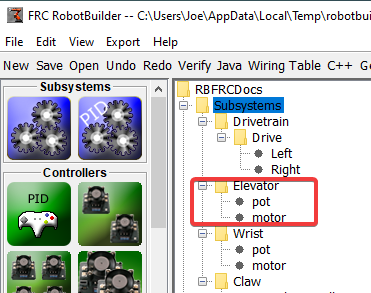
Each subsystem consists of a number of actuators, sensors and controllers that it uses to perform its operations. These sensors and actuators are added to the subsystem with which they are associated. Each of the sensors and actuators comes from the RobotBuilder palette and is dragged to the appropriate subsystem. For each, there are usually other properties that must be set such as port numbers and other parameters specific to the component.
In this example there is an Elevator subsystem that uses a motor and a potentiometer (motor and pot) that have been dragged to the Elevator subsystem.
Adding Commands That Describe Subsystem Goals
Commands are distinct goals that the robot will perform. These commands are added by dragging the command under the “Commands” folder. When creating a command, there are 7 choices (shown on the palette on the left of the picture):
Normal commands - these are the most flexible command, you have to write all of the code to perform the desired actions necessary to accomplish the goal.
Timed commands - these commands are a simplified version of a command that ends after a timeout
Instant commands - these commands are a simplified versio of a command that runs for one iteration and then ends
Command groups - these commands are a combination of other commands running both in a sequential order and in parallel. Use these to build up more complicated actions after you have a number of basic commands implemented.
Setpoint commands - setpoint commands move a PID Subsystem to a fixed setpoint, or the desired location.
PID commands - these commands have a built-in PID controller to be used with a regular subsystem.
Conditional commands - these commands select one of two commands to run at the time of initialization.
For more information see Creating a Command and Writing Command Code.
Testing each Command
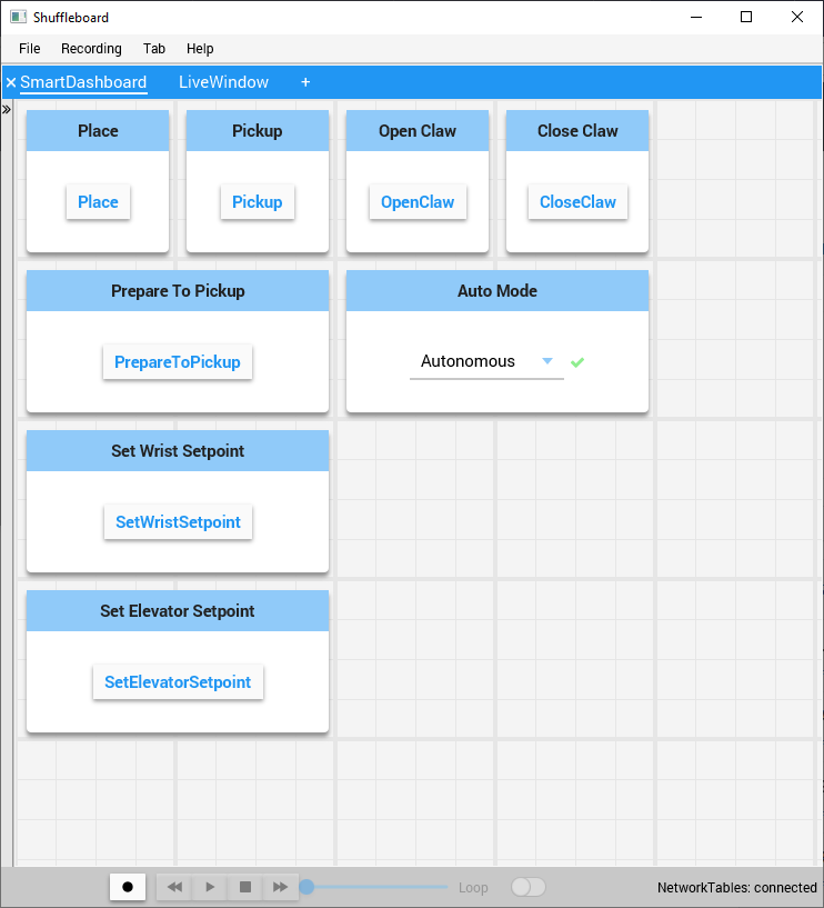
Each command can be run from Shuffleboard or SmartDashboard. This is useful for testing commands before you add them to the operator interface or to a command group. As long as you leave the “Button on SmartDashboard” property checked, a button will be created on the SmartDashboard. When you press the button, the command will run and you can check that it performs the desired action.
By creating buttons, each command can be tested individually. If all the commands work individually, you can be pretty sure that the robot will work as a whole.
For more information see Testing with Smartdashboard.
Adding Operator Interface Components
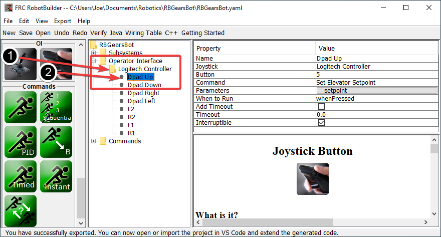
The operator interface consists of joysticks, gamepads and other HID input devices. You can add operator interface components (joysticks, joystick buttons) to your program in RobotBuilder. It will automatically generate code that will initialize all of the components and allow them to be connected to commands.
The operator interface components are dragged from the palette to the “Operator Interface” folder in the RobotBuilder program. First (1) add Joysticks to the program then put buttons under the associated joysticks (2) and give them meaningful names, like ShootButton.
Connecting the Commands to the Operator Interface
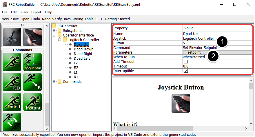
Commands can be associated with buttons so that when a button is pressed the command is scheduled. This should, for the most part, handle most of the tele-operated part of your robot program.
This is simply done by (1) adding the command to the JoystickButton object in the RobotBuilder program, then (2) setting the condition in which the command is scheduled.
For more information see Connecting the Operator Interface to a Command.
Developing Autonomous Commands
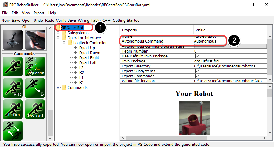
Commands make it simple to develop autonomous programs. You simply specify which command should run when the robot enters the autonomous period and it will automatically be scheduled. If you have tested commands as discussed above, this should simply be a matter of choosing which command should run.
Select the robot at the root of the RobotBuilder project (1), then edit the Autonomous Command property (2) to choose the command to run. It’s that simple!
For more information see Setting the Autonomous Commands.
Generating Code
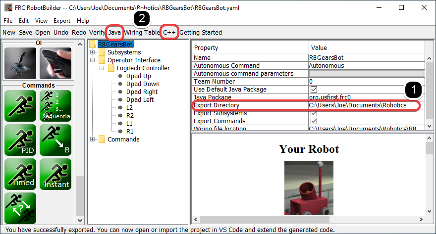
At any point in the process outlined above you can have RobotBuilder generate a C++ or Java program that will represent the project you have created. This is done by specifying the location of the project in the project properties (1), then clicking the appropriate toolbar button to generate the code (2).
For more information see Generating RobotBuilder Code.
Starting RobotBuilder
Note
RobotBuilder is a Java program and as such should be able to run on any platform that is supported by Java. We have been running RobotBuilder on macOS, Windows, and various versions of Linux successfully.
Getting RobotBuilder
RobotBuilder is downloaded as part of the WPILib Offline Installer. For more information, see the Windows/macOS/Linux installation guides
Option 1 - Starting from Visual Studio Code
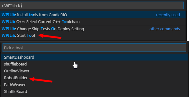
Press Ctrl+Shift+P and type “WPILib” or click the WPILib logo in the top right to launch the WPILib Command Palette. Select Start Tool, then select Robot Builder.
Option 2 - Shortcuts
Shortcuts are installed to the Windows Start Menu and the 2022 WPILib Tools folder on the desktop.
Option 3 - Running from the Script
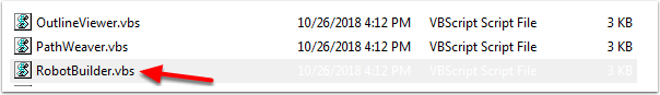
The install process installs the tools to ~/wpilib/YYYY/tools (where YYYY is the year and ~ is C:\Users\Public on Windows).
Inside this folder you will find .vbs (Windows) and .py (macOS/Linux) files that you can use to launch each tool. These scripts help launch the tools using the correct JDK and are what you should use to launch the tools.
RobotBuilder User Interface
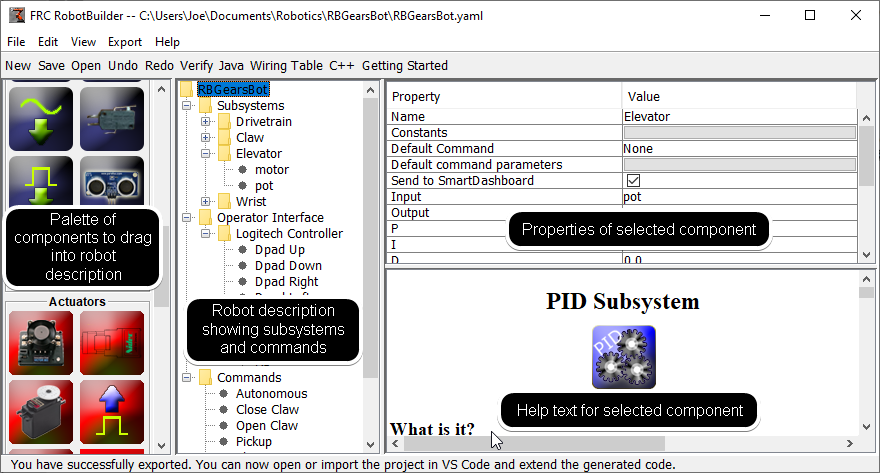
RobotBuilder has a user interface designed for rapid development of robot programs. Almost all operations are performed by drag-and-drop or selecting options from drop-down lists.
Dragging Items from the Palette to the Robot Description
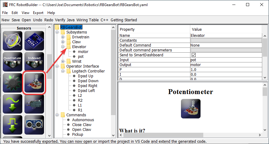
You can drag items from the palette to the robot description by starting the drag on the palette item and ending on the container where you would like the item to be located. In this example, dropping a potentiometer to the Elevator subsystem.
Adding Components using the Right-Click Context Menu
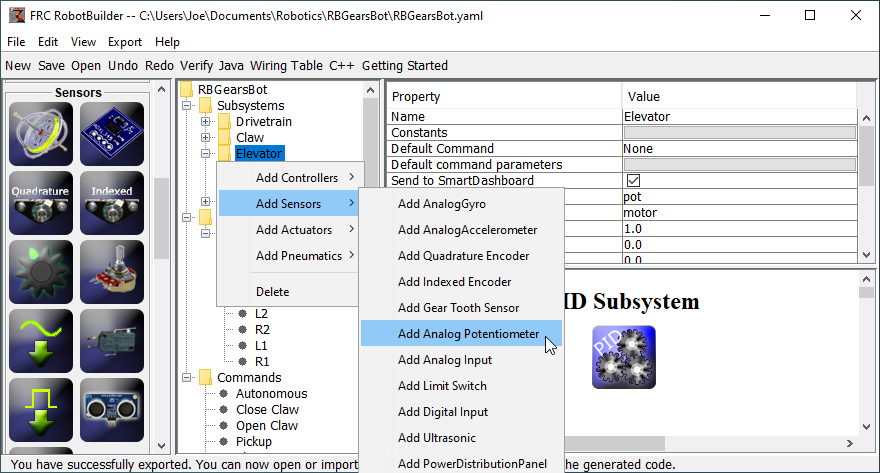
A shortcut method of adding items to the robot description is to right-click on the container object (Elevator) and select the item that should be added (Potentiometer). This is identical to using drag and drop but might be easier for some people.
Editing Properties of Robot Description Items
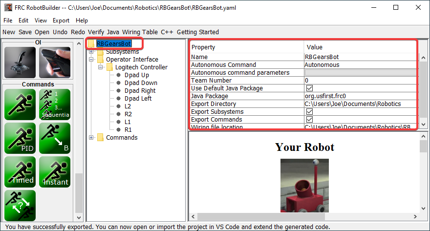
The properties for a selected item will appear in the properties viewer. The properties can be edited by selecting the value in the right hand column.
Using the Menu System
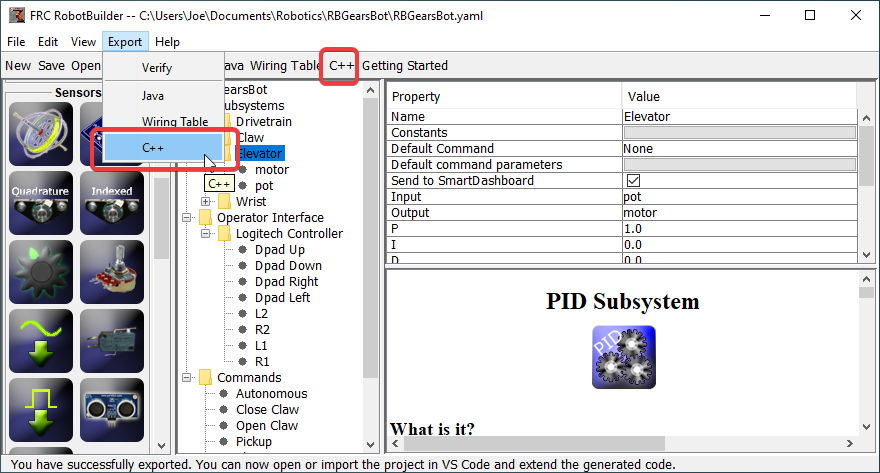
Operations for RobotBuilder can either be selected through the menu system or the equivalent item (if it is available) from the toolbar.
Setting up the Robot Project
The RobotBuilder program has some default properties that need to be set up so the generated program and other generated files work properly. This setup information is stored in the properties for robot description (the first line).
Robot Project Properties
The properties that describe the robot are:
Name - The name of the robot project that is created
Autonomous Command - the command that will run by default when the program is placed in autonomous mode
Autonomous Command Parameters - Parameters for the Autonomous Command
Team Number - The team number for the project, which will be used to locate the robot when deploying code.
Use Default Java Package - If checked RobotBuilder will use the default package (frc.robot). Otherwise you can specify a custom package name to be used.
Java Package - The name of the generated Java package used when generating the project code
Export Directory - The folder that the project is generated into when Export to Java or C++ is selected
Export Subsystems - Checked if RobotBuilder should export the Subsystem classes from your project
Export Commands - Checked if RobotBuilder should export the Command classes from your project
Wiring File location - the location of the html file to generate that contains the wiring diagram for your robot
Desktop Support - Enables unit test and simulation. While WPILib supports this, third party software libraries may not. If libraries do not support desktop, then your code may not compile or may crash. It should be left unchecked unless unit testing or simulation is needed and all libraries support it.
Using Source Control with the RobotBuilder Project
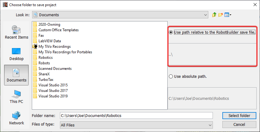
When using source control the project will typically be used on a number of computers and the path to the project directory might be different from one users computer to another. If the RobotBuilder project file is stored using an absolute path, it will typically contain the user name and won’t be usable across multiple computers. To make this work, select “relative path” and specify the path as an directory offset from the project files. In the above example, the project file is stored in the folder just above the project files in the file hierarchy. In this case, the user name is not part of the path and it will be portable across all of your computers.
Creating a Subsystem
Subsystems are classes that encapsulate (or contain) all the data and code that make a subsystem on your robot operate. The first step in creating a robot program with the RobotBuilder is to identify and create all the subsystems on the robot. Examples of subsystems are grippers, ball collectors, the drive base, elevators, arms, etc. Each subsystem contains all the sensors and actuators that are used to make it work. For example, an elevator might have a Victor SPX motor controller and a potentiometer to provide feedback of the robot position.
Creating a Subsystem using the Palette
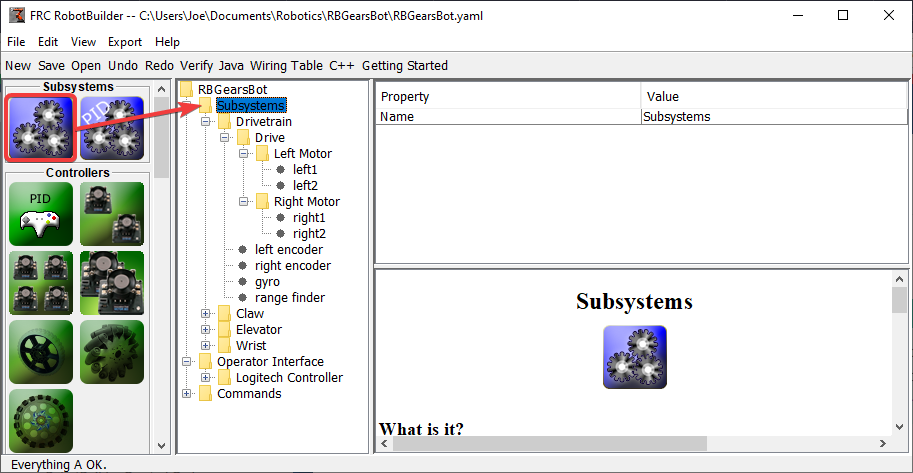
Drag the subsystem icon from the palette to the Subsystems folder in the robot description to create a subsystem class.
Creating a Subsystem using the Context Menu
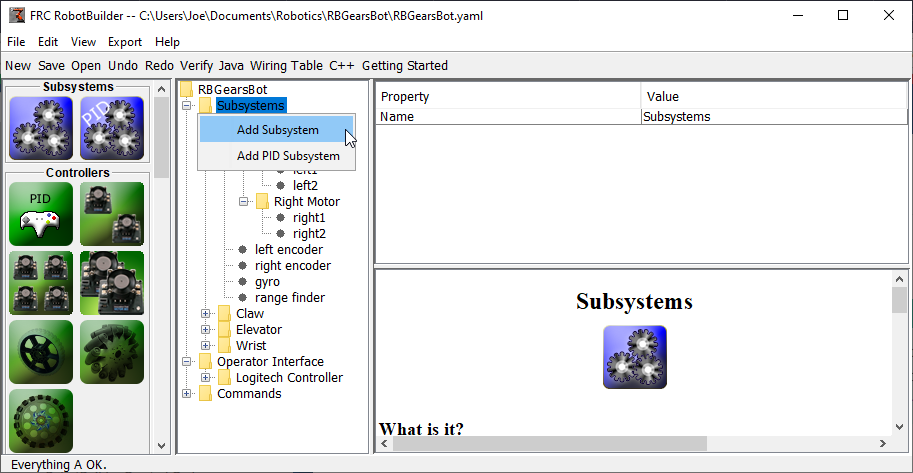
Right-click on the Subsystem folder in the robot description to add a subsystem to that folder.
Name the Subsystem
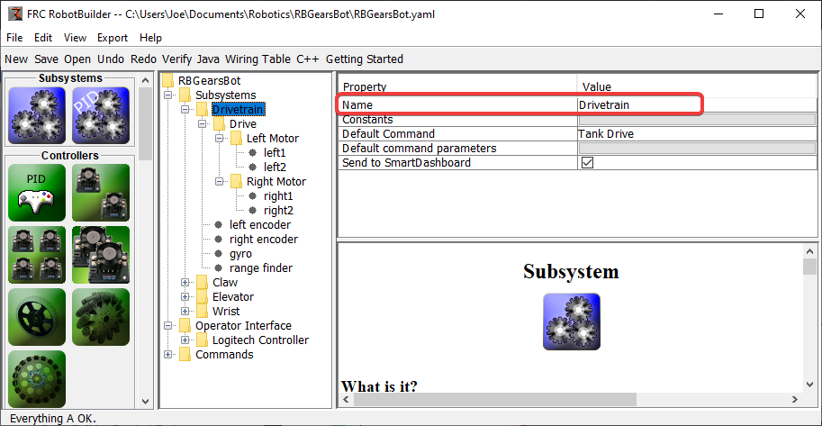
After creating the subsystem by either dragging or using the context menu as described above, simply type the name you would like to give the subsystem. The name can be multiple words separated by spaces, RobotBuilder will concatenate the words to make a proper Java or C++ class name for you.
Adding Constants
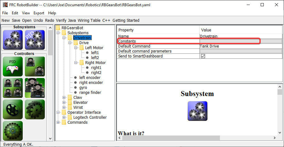
Constants are very useful to reduce the amount of magic numbers in your code. In subsystems, they can be used to keep track of certain values, such as sensor values for specific heights of an elevator, or the speed at which to drive the robot.
By default, there will be no constants in a subsystem. Press the button next to “Constants” to open a dialog to create some.
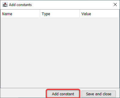
Add Constants
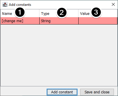
The name of the constant. Change this to something descriptive. In this example of a drivetrain some good constants might be “PlaceDistance” and “BackAwayDistance”.
The type of the constant. This will most likely be a double, but you can choose from one of: String, double, int, long, boolean, or byte.
The value of the constant.
Saving Constants
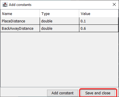
After adding constants and setting their values, just press “Save and close” to save the constants and close the dialog. If you don’t want to save, press the exit button on the top of the window.
After Saving
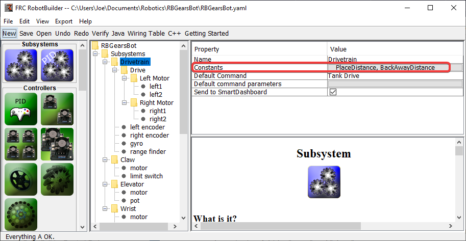
After saving constants, the names will appear in the “Constants” button in the subsystem properties.
Dragging Actuators/Sensors into the Subsystem
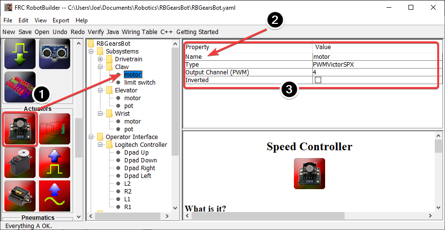
There are three steps to adding components to a subsystem:
Drag actuators or sensors from the palette into the subsystem as required.
Give the actuator or sensor a meaningful name
Edit the properties such as module numbers and channel numbers for each item in the subsystem.
RobotBuilder will automatically use incrementing channel numbers for each module on the robot. If you haven’t yet wired the robot you can just let RobotBuilder assign unique channel numbers for each sensor or actuator and wire the robot according to the generating wiring table.
This just creates the subsystem in RobotBuilder, and will subsequently generate skeleton code for the subsystem. To make it actually operate your robot please refer to Writing Code for a Subsystem.
Creating a Command
Commands are classes you create that provide behaviors or actions for your subsystems. The subsystem class should set the operation of the subsystem, like MoveElevator to start the elevator moving, or ElevatorToSetPoint to set the elevator’s PID setpoint. The commands initiate the subsystem operation and keep track of when it is finished.
Drag the Command to the Commands Folder
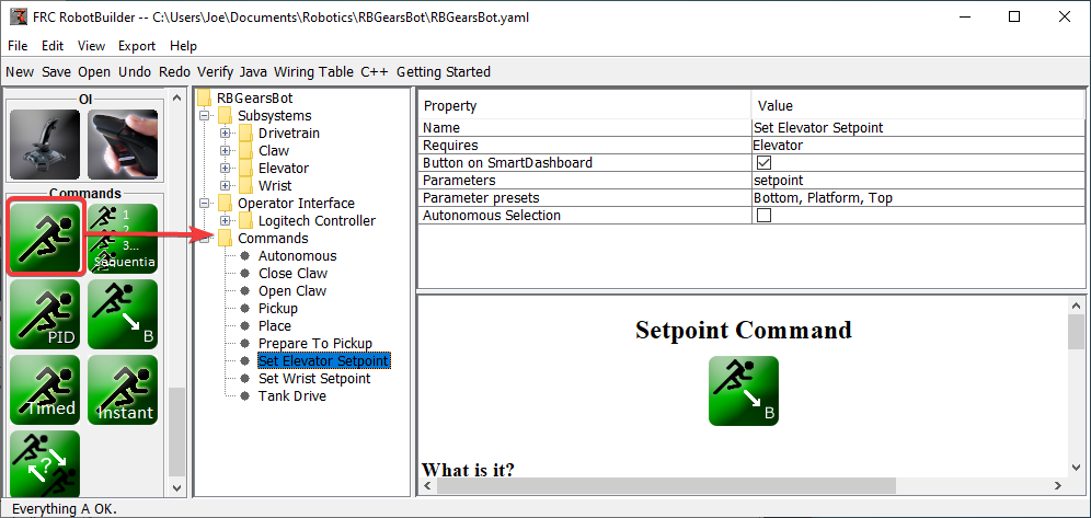
Simple commands can be dragged from the palette to the robot description. The command will be created under the Commands folder.
Creating Commands using the Context Menu
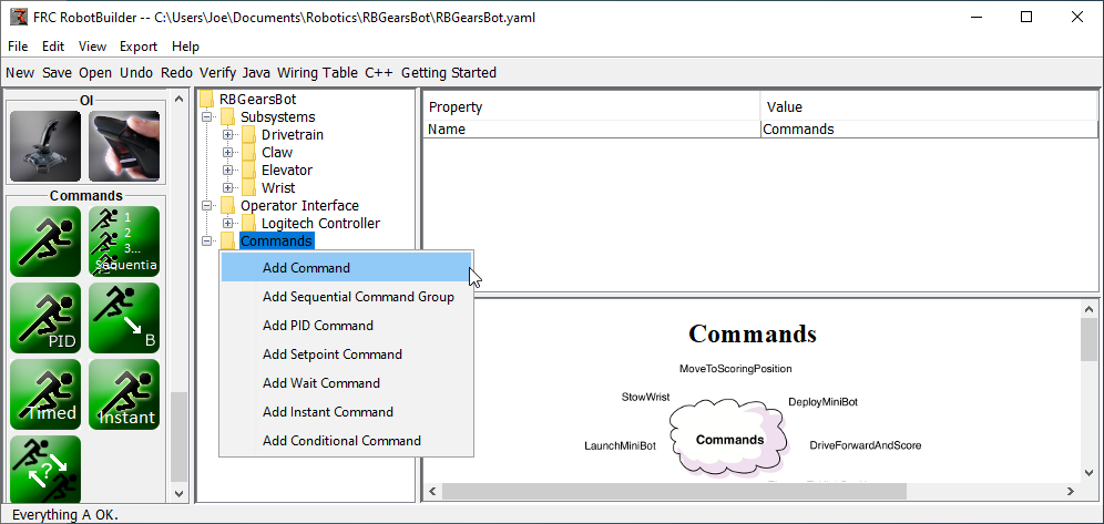
You can also create commands using the right-click context menu on the Command folder in the robot description.
Configuring the Command
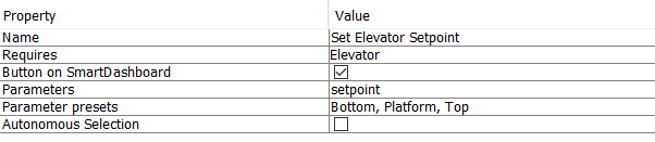
Name the command with something meaningful that describes what the command will do. Commands should be named as if they were in code, although there can be spaces between words.
Set the subsystem that is required by this command. When this command is scheduled, it will automatically stop any command currently running that also requires this command. If a command to open the claw is currently running (requiring the claw subsystem) and the close claw command is scheduled, it will immediately stop opening and start closing.
Tell RobotBuilder if it should create buttons on the SmartDashboard for the command. A button will be created for each parameter preset.
Set the parameters this command takes. A single command with parameters can do the same thing as two or more commands that do not take parameters. For example, “Drive Forward”, “Drive Backward”, and “Drive Distance” commands can be consolidated into a single command that takes values for direction and distance.
Set presets for parameters. These can be used elsewhere in RobotBuilder when using the command, such as binding it to a joystick button or setting the default command for a subsystem.
Run When Disabled. Allows the command to run when the robot is disabled. However, any actuators commanded while disabled will not actuate.
Autonomous Selection. Whether the command should be added to the Sendable Chooser so that it can be selected for autonomous.
Setpoint commands come with a single parameter (‘setpoint’, of type double); parameters cannot be added, edited, or deleted for setpoint commands.
Adding and Editing Parameters
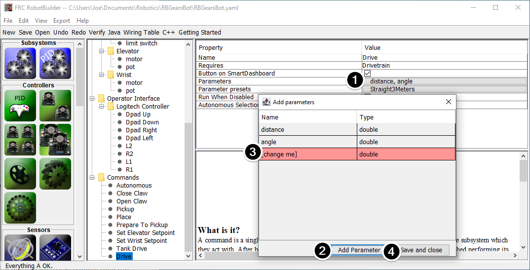
To add or edit parameters:
Click the button in the Value column of the property table
Press the Add Parameter button to add a parameter
A parameter that has just been added. The name defaults to [change me] and the type defaults to String. The default name is invalid, so you will have to change it before exporting. Double click the Name cell to start changing the name. Double click the Type cell to select the type.
Save and close button will save all changes and close the window.
Rows can be reordered simply by dragging, and can be deleted by selecting them and pressing delete or backspace.
Adding and Editing Parameter Presets
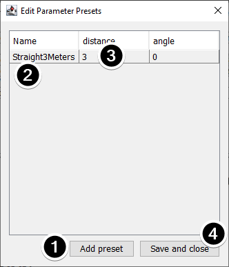
Click Add parameter set to add a new preset.
Change the name of the preset to something descriptive. The presets in this example are for opening and closing the gripper subsystem.
Change the value of the parameter(s) for the preset. You can either type a value in (e.g. “3.14”) or select from constants defined in the subsystem that the command requires. Note that the type of the constant has to be the same type as the parameter – you can’t have an int-type constant be passed to a double-type parameter, for example
Click Save and close to save changes and exit the dialog; to exit without saving, press the exit button in the top bar of the window.
Setting the Autonomous Commands
Since a command is simply one or more actions (behaviors) that the robot performs, it makes sense to describe the autonomous operation of a robot as a command. While it could be a single command, it is more likely going to be a command group (a group of commands that happen together).
RobotBuilder generates code for a Sendable Chooser which allows the autonomous command to run to be chosen from the dashboard.
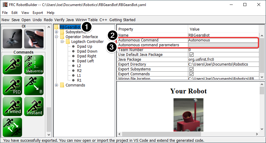
To designate the default autonomous command that runs if another command is not selected on the dashboard:
Select the robot in the robot program description
Fill in the Autonomous command field with the command that should run when the robot is placed in autonomous mode. This is a drop-down field and will give you the option to select any command that has been defined.
Set the parameters the command takes, if any.
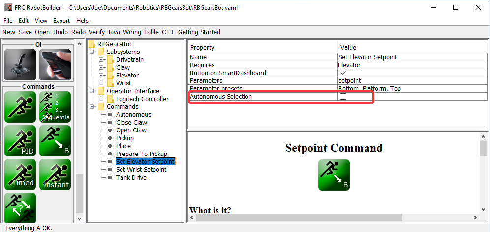
To select commands to add as options to the Sendable Chooser, select the Autonomous Selection check box.
When the robot is put into autonomous mode, the chosen Autonomous command will be scheduled.
Using Shuffleboard to Test a Command
Commands are easily tested by adding a button to Shuffleboard/SmartDashboard to trigger the command. In this way, no integration with the rest of the robot program is necessary and commands can easily be independently tested. This is the easiest way to verify commands since with a single line of code in your program, a button can be created on Shuffleboard that will run the command. These buttons can then be left in place to verify subsystems and command operations in the future.
This has the added benefit of accommodating multiple programmers, each writing commands. As the code is checked into the main robot project, the commands can be individually tested.
Creating the Button on Shuffleboard
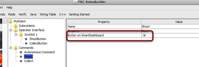
The button is created on the SmartDashboard by putting an instance of the command from the robot program to the dashboard. This is such a common operation that it has been added to RobotBuilder as a checkbox. When writing your commands, be sure that the box is checked, and buttons will be automatically generated for you.
Operating the Buttons
The buttons will be generated automatically and will appear on the dashboard screen. You can rearrange the buttons on Shuffleboard. In this example there are a number of commands, each with an associated button for testing. Pressing the commands button will run the command. Once it is pressed, pressing again it will interrupt the command causing the Interrupted() method to be called.
Adding Commands Manually
SmartDashboard.putData("Autonomous Command", new AutonomousCommand());
SmartDashboard.putData("Open Claw", new OpenClaw(m_claw);
SmartDashboard.putData("Close Claw", new CloseClaw(m_claw));
SmartDashboard::PutData("Autonomous Command", new AutonomousCommand());
SmartDashboard::PutData("Open Claw", new OpenClaw(&m_claw));
SmartDashboard::PutData("Close Claw", new CloseClaw(&m_claw));
Commands can be added to the Shuffleboard manually by writing the code yourself. This is done by passing instances of the command to the PutData method along with the name that should be associated with the button on the Shuffleboard. These instances are scheduled whenever the button is pressed. The result is exactly the same as RobotBuilder generated code, although clicking the checkbox in RobotBuilder is much easier than writing all the code by hand.
Connecting the Operator Interface to a Command
Commands handle the behaviors for your robot. The command starts a subsystem to some operating mode like raising and elevator and continues running until it reaches some setpoint or timeout. The command then handles waiting for the subsystem to finish. That way commands can run in sequence to develop more complex behaviors.
RobotBuilder will also generate code to schedule a command to run whenever a button on your operator interface is pressed. You can also write code to run a command when a particular trigger condition has happened.
Run a Command with a Button Press
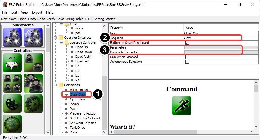
In this example we want to schedule the “Close Claw” command to run whenever the dpad right direction button is pressed on a logitech gamepad (button 6) is pressed.
The command to run is called “Close Claw” and its function is to close the claw of the robot
Notice that the command requires the Claw subsystem. This will ensure that this command starts running even if there was another operation happening at the same time that used the claw. In this case the previous command would be interrupted.
Parameters make it possible for one command to do multiple things; presets let you define values you pass to the command and reuse them
Adding the Joystick to the Robot Program
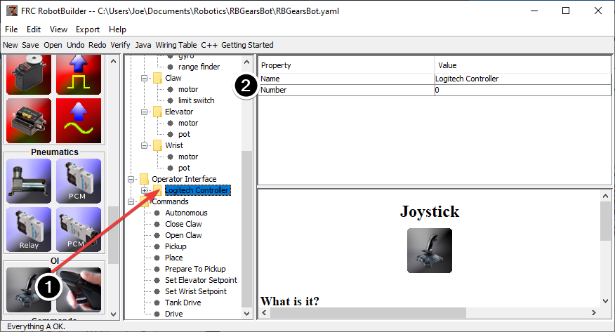
Add the joystick to the robot program
Drag the joystick to the Operator Interface folder in the robot program
Name the joystick so that it reflects the use of the joystick and set the USB port number
Linking a Button to the “Move Elevator” Command
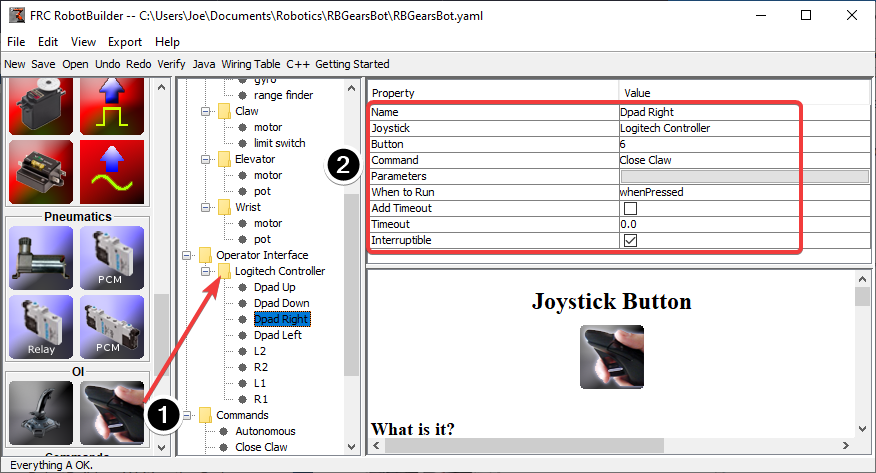
Add the button that should be pressed to the program
Drag the joystick button to the Joystick (Logitech Controller) so that it’s under the joystick
Set the properties for the button: the button number, the command to run when the button is pressed, parameters the command takes, and the “When to run” property to “whenPressed” to indicate that the command should run whenever the joystick button is pressed.
Note
Joystick buttons must be dragged to (under) a Joystick. You must have a joystick in the Operator Interface folder before adding buttons.
RobotBuilder Created Code
The Layout of a RobotBuilder Generated Project
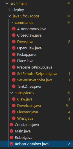
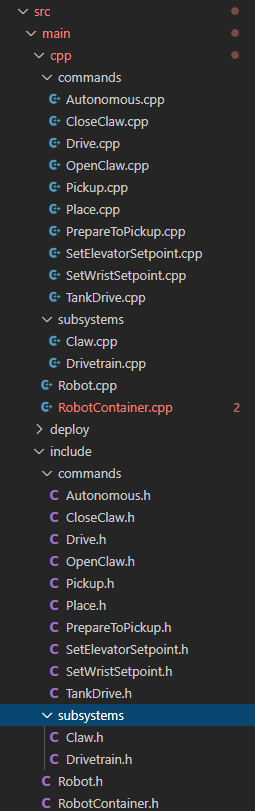
A RobotBuilder generated project consists of a package (in Java) or a folder (in C++) for Commands and another for Subsystems. Each command or subsystem object is stored under those containers. At the top level of the project you’ll find the robot main program (RobotContainer.java/C++).
For more information on the organization of a Command Based robot, see Structuring a Command-Based Robot Project
Autogenerated Code
// BEGIN AUTOGENERATED CODE, SOURCE=ROBOTBUILDER ID=AUTONOMOUS
m_chooser.setDefaultOption("Autonomous", new Autonomous());
// END AUTOGENERATED CODE, SOURCE=ROBOTBUILDER ID=AUTONOMOUS
SmartDashboard.putData("Auto Mode", m_chooser);
// BEGIN AUTOGENERATED CODE, SOURCE=ROBOTBUILDER ID=AUTONOMOUS
m_chooser.SetDefaultOption("Autonomous", new Autonomous());
// END AUTOGENERATED CODE, SOURCE=ROBOTBUILDER ID=AUTONOMOUS
frc::SmartDashboard::PutData("Auto Mode", &m_chooser);
When the robot description is modified and code is re-exported RobotBuilder is designed to not modify any changes you made to the file, thus preserving your code. This makes RobotBuilder a full-lifecycle tool. To know what code is OK to be modified by RobotBuilder, it generates sections that will potentially have to be rewritten delimited with some special comments. These comments are shown in the example above. Don’t add any code within these comment blocks, it will be rewritten next time the project is exported from RobotBuilder.
If code inside one of these blocks must be modified, the comments can be removed, but this will prevent further updates from happening later. In the above example, if the //BEGIN and //END comments were removed, then later another required subsystem was added in RobotBuilder, it would not be generated on that next export.
// ROBOTBUILDER TYPE: Robot.
// ROBOTBUILDER TYPE: Robot.
Additionally, each file has a comment defining the type of file. If this is modified or deleted, RobotBuilder will completely regenerate the file deleting any code added both inside and outside the AUTOGENERATED CODE blocks.
Main Robot Program
11// ROBOTBUILDER TYPE: Robot.
12
13package frc.robot;
14
15import edu.wpi.first.hal.FRCNetComm.tInstances;
16import edu.wpi.first.hal.FRCNetComm.tResourceType;
17import edu.wpi.first.hal.HAL;
18import edu.wpi.first.wpilibj.TimedRobot;
19import edu.wpi.first.wpilibj2.command.Command;
20import edu.wpi.first.wpilibj2.command.CommandScheduler;
21
22/**
23 * The VM is configured to automatically run this class, and to call the
24 * functions corresponding to each mode, as described in the TimedRobot
25 * documentation. If you change the name of this class or the package after
26 * creating this project, you must also update the build.properties file in
27 * the project.
28 */
29public class Robot extends TimedRobot { // (1)
30
31 private Command m_autonomousCommand;
32
33 private RobotContainer m_robotContainer;
34
35 /**
36 * This function is run when the robot is first started up and should be
37 * used for any initialization code.
38 */
39 @Override
40 public void robotInit() {
41 // Instantiate our RobotContainer. This will perform all our button bindings, and put our
42 // autonomous chooser on the dashboard.
43 m_robotContainer = RobotContainer.getInstance();
44 HAL.report(tResourceType.kResourceType_Framework, tInstances.kFramework_RobotBuilder);
45 }
46
47 /**
48 * This function is called every robot packet, no matter the mode. Use this for items like
49 * diagnostics that you want ran during disabled, autonomous, teleoperated and test.
50 *
51 * <p>This runs after the mode specific periodic functions, but before
52 * LiveWindow and SmartDashboard integrated updating.
53 */
54 @Override
55 public void robotPeriodic() {
56 // Runs the Scheduler. This is responsible for polling buttons, adding newly-scheduled
57 // commands, running already-scheduled commands, removing finished or interrupted commands,
58 // and running subsystem periodic() methods. This must be called from the robot's periodic
59 // block in order for anything in the Command-based framework to work.
60 CommandScheduler.getInstance().run(); // (2)
61 }
62
63
64 /**
65 * This function is called once each time the robot enters Disabled mode.
66 */
67 @Override
68 public void disabledInit() {
69 }
70
71 @Override
72 public void disabledPeriodic() {
73 }
74
75 /**
76 * This autonomous runs the autonomous command selected by your {@link RobotContainer} class.
77 */
78 @Override
79 public void autonomousInit() {
80 m_autonomousCommand = m_robotContainer.getAutonomousCommand(); // (3)
81
82 // schedule the autonomous command (example)
83 if (m_autonomousCommand != null) {
84 m_autonomousCommand.schedule();
85 }
86 }
87
88 /**
89 * This function is called periodically during autonomous.
90 */
91 @Override
92 public void autonomousPeriodic() {
93 }
94
95 @Override
96 public void teleopInit() {
97 // This makes sure that the autonomous stops running when
98 // teleop starts running. If you want the autonomous to
99 // continue until interrupted by another command, remove
100 // this line or comment it out.
101 if (m_autonomousCommand != null) {
102 m_autonomousCommand.cancel();
103 }
104 }
105
106 /**
107 * This function is called periodically during operator control.
108 */
109 @Override
110 public void teleopPeriodic() {
111 }
112
113 @Override
114 public void testInit() {
115 // Cancels all running commands at the start of test mode.
116 CommandScheduler.getInstance().cancelAll();
117 }
118
119 /**
120 * This function is called periodically during test mode.
121 */
122 @Override
123 public void testPeriodic() {
124 }
125
126}
11// ROBOTBUILDER TYPE: Robot.
12#pragma once
13
14#include <frc/TimedRobot.h>
15#include <frc2/command/Command.h>
16
17#include "RobotContainer.h"
18
19class Robot : public frc::TimedRobot { // {1}
20 public:
21 void RobotInit() override;
22 void RobotPeriodic() override;
23 void DisabledInit() override;
24 void DisabledPeriodic() override;
25 void AutonomousInit() override;
26 void AutonomousPeriodic() override;
27 void TeleopInit() override;
28 void TeleopPeriodic() override;
29 void TestPeriodic() override;
30
31 private:
32 // Have it null by default so that if testing teleop it
33 // doesn't have undefined behavior and potentially crash.
34 frc2::Command* m_autonomousCommand = nullptr;
35
36 RobotContainer* m_container = RobotContainer::GetInstance();
37};
11// ROBOTBUILDER TYPE: Robot.
12
13#include "Robot.h"
14
15#include <frc/smartdashboard/SmartDashboard.h>
16#include <frc2/command/CommandScheduler.h>
17
18void Robot::RobotInit() {}
19
20/**
21 * This function is called every robot packet, no matter the mode. Use
22 * this for items like diagnostics that you want to run during disabled,
23 * autonomous, teleoperated and test.
24 *
25 * <p> This runs after the mode specific periodic functions, but before
26 * LiveWindow and SmartDashboard integrated updating.
27 */
28void Robot::RobotPeriodic() { frc2::CommandScheduler::GetInstance().Run(); } // (2)
29
30/**
31 * This function is called once each time the robot enters Disabled mode. You
32 * can use it to reset any subsystem information you want to clear when the
33 * robot is disabled.
34 */
35void Robot::DisabledInit() {}
36
37void Robot::DisabledPeriodic() {}
38
39/**
40 * This autonomous runs the autonomous command selected by your {@link
41 * RobotContainer} class.
42 */
43void Robot::AutonomousInit() {
44 m_autonomousCommand = m_container->GetAutonomousCommand(); // {3}
45
46 if (m_autonomousCommand != nullptr) {
47 m_autonomousCommand->Schedule();
48 }
49}
50
51void Robot::AutonomousPeriodic() {}
52
53void Robot::TeleopInit() {
54 // This makes sure that the autonomous stops running when
55 // teleop starts running. If you want the autonomous to
56 // continue until interrupted by another command, remove
57 // this line or comment it out.
58 if (m_autonomousCommand != nullptr) {
59 m_autonomousCommand->Cancel();
60 m_autonomousCommand = nullptr;
61 }
62}
63
64/**
65 * This function is called periodically during operator control.
66 */
67void Robot::TeleopPeriodic() {}
68
69/**
70 * This function is called periodically during test mode.
71 */
72void Robot::TestPeriodic() {}
73
74#ifndef RUNNING_FRC_TESTS
75int main() { return frc::StartRobot<Robot>(); }
76#endif
This is the main program generated by RobotBuilder. There are a number of parts to this program (highlighted sections):
This class extends TimedRobot. TimedRobot will call your
autonomousPeriodic()andteleopPeriodic()methods every 20ms.In the robotPeriodic method which is called every 20ms, make one scheduling pass.
The autonomous command provided is scheduled at the start of autonomous in the
autonomousInit()method and canceled at the end of the autonomous period inteleopInit().
RobotContainer
11// ROBOTBUILDER TYPE: RobotContainer.
12
13package frc.robot;
14
15import frc.robot.commands.*;
16import frc.robot.subsystems.*;
17import edu.wpi.first.wpilibj.smartdashboard.SendableChooser;
18import edu.wpi.first.wpilibj.smartdashboard.SmartDashboard;
19
20// BEGIN AUTOGENERATED CODE, SOURCE=ROBOTBUILDER ID=IMPORTS
21import edu.wpi.first.wpilibj2.command.Command;
22import edu.wpi.first.wpilibj2.command.InstantCommand;
23import edu.wpi.first.wpilibj.Joystick;
24import edu.wpi.first.wpilibj2.command.button.JoystickButton;
25import frc.robot.subsystems.*;
26
27 // END AUTOGENERATED CODE, SOURCE=ROBOTBUILDER ID=IMPORTS
28
29
30/**
31 * This class is where the bulk of the robot should be declared. Since Command-based is a
32 * "declarative" paradigm, very little robot logic should actually be handled in the {@link Robot}
33 * periodic methods (other than the scheduler calls). Instead, the structure of the robot
34 * (including subsystems, commands, and button mappings) should be declared here.
35 */
36public class RobotContainer {
37
38 private static RobotContainer m_robotContainer = new RobotContainer();
39
40 // BEGIN AUTOGENERATED CODE, SOURCE=ROBOTBUILDER ID=DECLARATIONS
41// The robot's subsystems
42 public final Wrist m_wrist = new Wrist(); // {1}
43 public final Elevator m_elevator = new Elevator();
44 public final Claw m_claw = new Claw();
45 public final Drivetrain m_drivetrain = new Drivetrain();
46
47// Joysticks
48private final Joystick joystick2 = new Joystick(2); // {3}
49private final Joystick joystick1 = new Joystick(1);
50private final Joystick logitechController = new Joystick(0);
51
52 // END AUTOGENERATED CODE, SOURCE=ROBOTBUILDER ID=DECLARATIONS
53
54
55 // A chooser for autonomous commands
56 SendableChooser<Command> m_chooser = new SendableChooser<>();
57
58 /**
59 * The container for the robot. Contains subsystems, OI devices, and commands.
60 */
61 private RobotContainer() {
62 // BEGIN AUTOGENERATED CODE, SOURCE=ROBOTBUILDER ID=SMARTDASHBOARD
63 // Smartdashboard Subsystems
64 SmartDashboard.putData(m_wrist);
65 SmartDashboard.putData(m_elevator);
66 SmartDashboard.putData(m_claw);
67 SmartDashboard.putData(m_drivetrain);
68
69
70 // SmartDashboard Buttons
71 SmartDashboard.putData("Close Claw", new CloseClaw( m_claw )); // {6}
72 SmartDashboard.putData("Open Claw: OpenTime", new OpenClaw(1.0, m_claw));
73 SmartDashboard.putData("Pickup", new Pickup());
74 SmartDashboard.putData("Place", new Place());
75 SmartDashboard.putData("Prepare To Pickup", new PrepareToPickup());
76 SmartDashboard.putData("Set Elevator Setpoint: Bottom", new SetElevatorSetpoint(0, m_elevator));
77 SmartDashboard.putData("Set Elevator Setpoint: Platform", new SetElevatorSetpoint(0.2, m_elevator));
78 SmartDashboard.putData("Set Elevator Setpoint: Top", new SetElevatorSetpoint(0.3, m_elevator));
79 SmartDashboard.putData("Set Wrist Setpoint: Horizontal", new SetWristSetpoint(0, m_wrist));
80 SmartDashboard.putData("Set Wrist Setpoint: Raise Wrist", new SetWristSetpoint(-45, m_wrist));
81 SmartDashboard.putData("Drive: Straight3Meters", new Drive(3, 0, m_drivetrain));
82 SmartDashboard.putData("Drive: Place", new Drive(Drivetrain.PlaceDistance, Drivetrain.BackAwayDistance, m_drivetrain));
83
84 // END AUTOGENERATED CODE, SOURCE=ROBOTBUILDER ID=SMARTDASHBOARD
85 // Configure the button bindings
86 configureButtonBindings();
87
88 // Configure default commands
89 // BEGIN AUTOGENERATED CODE, SOURCE=ROBOTBUILDER ID=SUBSYSTEM_DEFAULT_COMMAND
90 m_drivetrain.setDefaultCommand(new TankDrive( m_drivetrain ) ); // {5}
91
92
93 // END AUTOGENERATED CODE, SOURCE=ROBOTBUILDER ID=SUBSYSTEM_DEFAULT_COMMAND
94
95 // Configure autonomous sendable chooser
96 // BEGIN AUTOGENERATED CODE, SOURCE=ROBOTBUILDER ID=AUTONOMOUS
97
98 m_chooser.setDefaultOption("Autonomous", new Autonomous()); // {2}
99
100 // END AUTOGENERATED CODE, SOURCE=ROBOTBUILDER ID=AUTONOMOUS
101
102 SmartDashboard.putData("Auto Mode", m_chooser);
103 }
104
105 public static RobotContainer getInstance() {
106 return m_robotContainer;
107 }
108
109 /**
110 * Use this method to define your button->command mappings. Buttons can be created by
111 * instantiating a {@link GenericHID} or one of its subclasses ({@link
112 * edu.wpi.first.wpilibj.Joystick} or {@link XboxController}), and then passing it to a
113 * {@link edu.wpi.first.wpilibj2.command.button.JoystickButton}.
114 */
115 private void configureButtonBindings() {
116 // BEGIN AUTOGENERATED CODE, SOURCE=ROBOTBUILDER ID=BUTTONS
117// Create some buttons
118final JoystickButton r1 = new JoystickButton(logitechController, 12); // {4}
119r1.whenPressed(new Autonomous() ,true);
120 SmartDashboard.putData("R1",new Autonomous() );
121
122final JoystickButton l1 = new JoystickButton(logitechController, 11);
123l1.whenPressed(new Place() ,true);
124 SmartDashboard.putData("L1",new Place() );
125
126final JoystickButton r2 = new JoystickButton(logitechController, 10);
127r2.whenPressed(new Pickup() ,true);
128 SmartDashboard.putData("R2",new Pickup() );
129
130final JoystickButton l2 = new JoystickButton(logitechController, 9);
131l2.whenPressed(new PrepareToPickup() ,true);
132 SmartDashboard.putData("L2",new PrepareToPickup() );
133
134final JoystickButton dpadLeft = new JoystickButton(logitechController, 8);
135dpadLeft.whenPressed(new OpenClaw(1.0, m_claw) ,true);
136 SmartDashboard.putData("Dpad Left",new OpenClaw(1.0, m_claw) );
137
138final JoystickButton dpadRight = new JoystickButton(logitechController, 6);
139dpadRight.whenPressed(new CloseClaw( m_claw ) ,true);
140 SmartDashboard.putData("Dpad Right",new CloseClaw( m_claw ) );
141
142final JoystickButton dpadDown = new JoystickButton(logitechController, 7);
143dpadDown.whenPressed(new SetElevatorSetpoint(0, m_elevator) ,true);
144 SmartDashboard.putData("Dpad Down",new SetElevatorSetpoint(0, m_elevator) );
145
146final JoystickButton dpadUp = new JoystickButton(logitechController, 5);
147dpadUp.whenPressed(new SetElevatorSetpoint(0.3, m_elevator) ,true);
148 SmartDashboard.putData("Dpad Up",new SetElevatorSetpoint(0.3, m_elevator) );
149
150
151
152 // END AUTOGENERATED CODE, SOURCE=ROBOTBUILDER ID=BUTTONS
153 }
154
155 // BEGIN AUTOGENERATED CODE, SOURCE=ROBOTBUILDER ID=FUNCTIONS
156public Joystick getLogitechController() {
157 return logitechController;
158 }
159
160public Joystick getJoystick1() {
161 return joystick1;
162 }
163
164public Joystick getJoystick2() {
165 return joystick2;
166 }
167
168
169 // END AUTOGENERATED CODE, SOURCE=ROBOTBUILDER ID=FUNCTIONS
170
171 /**
172 * Use this to pass the autonomous command to the main {@link Robot} class.
173 *
174 * @return the command to run in autonomous
175 */
176 public Command getAutonomousCommand() {
177 // The selected command will be run in autonomous
178 return m_chooser.getSelected();
179 }
180
181
182}
11// ROBOTBUILDER TYPE: RobotContainer.
12
13#pragma once
14
15// BEGIN AUTOGENERATED CODE, SOURCE=ROBOTBUILDER ID=INCLUDES
16#include <frc/smartdashboard/SendableChooser.h>
17#include <frc2/command/Command.h>
18
19#include "subsystems/Claw.h"
20#include "subsystems/Drivetrain.h"
21#include "subsystems/Elevator.h"
22#include "subsystems/Wrist.h"
23
24#include "commands/Autonomous.h"
25#include "commands/CloseClaw.h"
26#include "commands/Drive.h"
27#include "commands/OpenClaw.h"
28#include "commands/Pickup.h"
29#include "commands/Place.h"
30#include "commands/PrepareToPickup.h"
31#include "commands/SetElevatorSetpoint.h"
32#include "commands/SetWristSetpoint.h"
33#include "commands/TankDrive.h"
34#include <frc/Joystick.h>
35#include <frc2/command/button/JoystickButton.h>
36
37// END AUTOGENERATED CODE, SOURCE=ROBOTBUILDER ID=INCLUDES
38
39class RobotContainer {
40
41public:
42
43 frc2::Command* GetAutonomousCommand();
44 static RobotContainer* GetInstance();
45
46 // BEGIN AUTOGENERATED CODE, SOURCE=ROBOTBUILDER ID=PROTOTYPES
47// The robot's subsystems
48Drivetrain m_drivetrain; // {1}
49Claw m_claw;
50Elevator m_elevator;
51Wrist m_wrist;
52
53
54frc::Joystick* getJoystick2();
55frc::Joystick* getJoystick1();
56frc::Joystick* getLogitechController();
57
58 // END AUTOGENERATED CODE, SOURCE=ROBOTBUILDER ID=PROTOTYPES
59
60private:
61
62 RobotContainer();
63
64 // BEGIN AUTOGENERATED CODE, SOURCE=ROBOTBUILDER ID=DECLARATIONS
65// Joysticks
66frc::Joystick m_joystick2{2}; // {3}
67frc::Joystick m_joystick1{1};
68frc::Joystick m_logitechController{0};
69
70frc::SendableChooser<frc2::Command*> m_chooser;
71
72 // END AUTOGENERATED CODE, SOURCE=ROBOTBUILDER ID=DECLARATIONS
73
74Autonomous m_autonomousCommand;
75 static RobotContainer* m_robotContainer;
76
77 void ConfigureButtonBindings();
78};
11// ROBOTBUILDER TYPE: RobotContainer.
12
13#include "RobotContainer.h"
14#include <frc2/command/ParallelRaceGroup.h>
15#include <frc/smartdashboard/SmartDashboard.h>
16
17
18
19RobotContainer* RobotContainer::m_robotContainer = NULL;
20
21RobotContainer::RobotContainer() : m_autonomousCommand(
22 // BEGIN AUTOGENERATED CODE, SOURCE=ROBOTBUILDER ID=CONSTRUCTOR
23){
24
25
26
27 // END AUTOGENERATED CODE, SOURCE=ROBOTBUILDER ID=CONSTRUCTOR
28
29 // BEGIN AUTOGENERATED CODE, SOURCE=ROBOTBUILDER ID=SMARTDASHBOARD
30 // Smartdashboard Subsystems
31 frc::SmartDashboard::PutData(&m_wrist);
32 frc::SmartDashboard::PutData(&m_elevator);
33 frc::SmartDashboard::PutData(&m_claw);
34 frc::SmartDashboard::PutData(&m_drivetrain);
35
36
37 // SmartDashboard Buttons
38 frc::SmartDashboard::PutData("Close Claw", new CloseClaw( &m_claw )); // {6}
39 frc::SmartDashboard::PutData("Open Claw: OpenTime", new OpenClaw(1.0_s, &m_claw));
40 frc::SmartDashboard::PutData("Pickup", new Pickup());
41 frc::SmartDashboard::PutData("Place", new Place());
42 frc::SmartDashboard::PutData("Prepare To Pickup", new PrepareToPickup());
43 frc::SmartDashboard::PutData("Set Elevator Setpoint: Bottom", new SetElevatorSetpoint(0, &m_elevator));
44 frc::SmartDashboard::PutData("Set Elevator Setpoint: Platform", new SetElevatorSetpoint(0.2, &m_elevator));
45 frc::SmartDashboard::PutData("Set Elevator Setpoint: Top", new SetElevatorSetpoint(0.3, &m_elevator));
46 frc::SmartDashboard::PutData("Set Wrist Setpoint: Horizontal", new SetWristSetpoint(0, &m_wrist));
47 frc::SmartDashboard::PutData("Set Wrist Setpoint: Raise Wrist", new SetWristSetpoint(-45, &m_wrist));
48 frc::SmartDashboard::PutData("Drive: Straight3Meters", new Drive(3, 0, &m_drivetrain));
49 frc::SmartDashboard::PutData("Drive: Place", new Drive(Drivetrain::PlaceDistance, Drivetrain::BackAwayDistance, &m_drivetrain));
50
51 // END AUTOGENERATED CODE, SOURCE=ROBOTBUILDER ID=SMARTDASHBOARD
52
53 ConfigureButtonBindings();
54
55 // BEGIN AUTOGENERATED CODE, SOURCE=ROBOTBUILDER ID=DEFAULT-COMMANDS
56m_drivetrain.SetDefaultCommand(TankDrive( &m_drivetrain )); // {5}
57
58 // END AUTOGENERATED CODE, SOURCE=ROBOTBUILDER ID=DEFAULT-COMMANDS
59
60 // BEGIN AUTOGENERATED CODE, SOURCE=ROBOTBUILDER ID=AUTONOMOUS
61
62
63 m_chooser.SetDefaultOption("Autonomous", new Autonomous()); // {2}
64
65 // END AUTOGENERATED CODE, SOURCE=ROBOTBUILDER ID=AUTONOMOUS
66
67 frc::SmartDashboard::PutData("Auto Mode", &m_chooser);
68
69}
70
71RobotContainer* RobotContainer::GetInstance() {
72 if (m_robotContainer == NULL) {
73 m_robotContainer = new RobotContainer();
74 }
75 return(m_robotContainer);
76}
77
78void RobotContainer::ConfigureButtonBindings() {
79 // BEGIN AUTOGENERATED CODE, SOURCE=ROBOTBUILDER ID=BUTTONS
80
81frc2::JoystickButton m_dpadUp{&m_logitechController, 5}; // {4}
82frc2::JoystickButton m_dpadDown{&m_logitechController, 7};
83frc2::JoystickButton m_dpadRight{&m_logitechController, 6};
84frc2::JoystickButton m_dpadLeft{&m_logitechController, 8};
85frc2::JoystickButton m_l2{&m_logitechController, 9};
86frc2::JoystickButton m_r2{&m_logitechController, 10};
87frc2::JoystickButton m_l1{&m_logitechController, 11};
88frc2::JoystickButton m_r1{&m_logitechController, 12};
89
90m_dpadUp.WhenPressed(SetElevatorSetpoint(0.3, &m_elevator), true);
91m_dpadDown.WhenPressed(SetElevatorSetpoint(0, &m_elevator), true);
92m_dpadRight.WhenPressed(CloseClaw( &m_claw ), true);
93m_dpadLeft.WhenPressed(OpenClaw(1.0_s, &m_claw), true);
94m_l2.WhenPressed(PrepareToPickup(), true);
95m_r2.WhenPressed(Pickup(), true);
96m_l1.WhenPressed(Place(), true);
97m_r1.WhenPressed(Autonomous(), true);
98
99 // END AUTOGENERATED CODE, SOURCE=ROBOTBUILDER ID=BUTTONS
100}
101
102// BEGIN AUTOGENERATED CODE, SOURCE=ROBOTBUILDER ID=FUNCTIONS
103
104frc::Joystick* RobotContainer::getJoystick2() {
105 return &m_joystick2;
106}
107frc::Joystick* RobotContainer::getJoystick1() {
108 return &m_joystick1;
109}
110frc::Joystick* RobotContainer::getLogitechController() {
111 return &m_logitechController;
112}
113
114// END AUTOGENERATED CODE, SOURCE=ROBOTBUILDER ID=FUNCTIONS
115
116
117frc2::Command* RobotContainer::GetAutonomousCommand() {
118 // The selected command will be run in autonomous
119 return m_chooser.GetSelected();
120}
This is the RobotContainer generated by RobotBuilder which is where the subsystems and operator interface are defined. There are a number of parts to this program (highlighted sections):
Each of the subsystems is declared here. They can be passed as parameters to any commands that require them.
If there is an autonomous command provided in RobotBuilder robot properties, it is added to the Sendable Chooser to be selected on the dashboard.
The code for all the operator interface components is generated here.
In addition the code to link the OI buttons to commands that should run is also generated here.
Commands to be run on a subystem when no other commands are running are defined here.
Commands to be run via a dashboard are defined here.
RobotBuilder - Writing the Code
Generating Code for a Project
After you’ve set up your robot framework in RobotBuilder, you’ll need to export the code and load it into Visual Studio Code. This article describes the process for doing so.
Generate the Code for the Project
Verify that the Export Directory points to where you want (1) and then click Java or C++ (2) to generate a VS Code project or update code.
Open the Project in Visual Studio Code
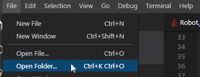
Open VS Code and select File -> Open Folder. Navigate to your Export location and click Select Folder.
Writing the Code for a Subsystem
Adding code to create an actual working subsystem is very straightforward. For simple subsystems that don’t use feedback it turns out to be extremely simple. In this section we will look at an example of a Claw subsystem. The Claw subsystem also has a limit switch to determine if an object is in the grip.
RobotBuilder Representation of the Claw Subsystem
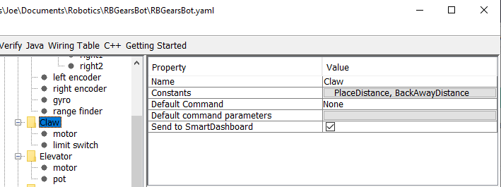
The claw at the end of a robot arm is a subsystem operated by a single VictorSPX Motor Controller. There are three things we want the motor to do, start opening, start closing, and stop moving. This is the responsibility of the subsystem. The timing for opening and closing will be handled by a command later in this tutorial. We will also define a method to get if the claw is gripping an object.
Adding Subsystem Capabilities
11// ROBOTBUILDER TYPE: Subsystem.
12
13package frc.robot.subsystems;
14
15
16import frc.robot.commands.*;
17import edu.wpi.first.wpilibj.livewindow.LiveWindow;
18import edu.wpi.first.wpilibj2.command.SubsystemBase;
19
20// BEGIN AUTOGENERATED CODE, SOURCE=ROBOTBUILDER ID=IMPORTS
21import edu.wpi.first.wpilibj.DigitalInput;
22import edu.wpi.first.wpilibj.motorcontrol.MotorController;
23import edu.wpi.first.wpilibj.motorcontrol.PWMVictorSPX;
24
25 // END AUTOGENERATED CODE, SOURCE=ROBOTBUILDER ID=IMPORTS
26
27
28/**
29 *
30 */
31public class Claw extends SubsystemBase {
32 // BEGIN AUTOGENERATED CODE, SOURCE=ROBOTBUILDER ID=CONSTANTS
33public static final double PlaceDistance = 0.1;
34public static final double BackAwayDistance = 0.6;
35
36 // END AUTOGENERATED CODE, SOURCE=ROBOTBUILDER ID=CONSTANTS
37
38 // BEGIN AUTOGENERATED CODE, SOURCE=ROBOTBUILDER ID=DECLARATIONS
39private PWMVictorSPX motor;
40private DigitalInput limitswitch;
41
42 // END AUTOGENERATED CODE, SOURCE=ROBOTBUILDER ID=DECLARATIONS
43
44 /**
45 *
46 */
47 public Claw() {
48 // BEGIN AUTOGENERATED CODE, SOURCE=ROBOTBUILDER ID=CONSTRUCTORS
49motor = new PWMVictorSPX(4);
50 addChild("motor",motor);
51 motor.setInverted(false);
52
53limitswitch = new DigitalInput(4);
54 addChild("limit switch", limitswitch);
55
56
57
58 // END AUTOGENERATED CODE, SOURCE=ROBOTBUILDER ID=CONSTRUCTORS
59 }
60
61 @Override
62 public void periodic() {
63 // This method will be called once per scheduler run
64
65 }
66
67 @Override
68 public void simulationPeriodic() {
69 // This method will be called once per scheduler run when in simulation
70
71 }
72
73 public void open() {
74 motor.set(1.0);
75 }
76
77 public void close() {
78 motor.set(-1.0);
79 }
80
81 public void stop() {
82 motor.set(0.0);
83 }
84
85 public boolean isGripping() {
86 return limitswitch.get();
87 }
88
89}
11// ROBOTBUILDER TYPE: Subsystem.
12
13// BEGIN AUTOGENERATED CODE, SOURCE=ROBOTBUILDER ID=INCLUDES
14#include "subsystems/Claw.h"
15#include <frc/smartdashboard/SmartDashboard.h>
16
17// END AUTOGENERATED CODE, SOURCE=ROBOTBUILDER ID=INCLUDES
18
19Claw::Claw(){
20 SetName("Claw");
21 // BEGIN AUTOGENERATED CODE, SOURCE=ROBOTBUILDER ID=DECLARATIONS
22 SetSubsystem("Claw");
23
24 AddChild("limit switch", &m_limitswitch);
25
26
27 AddChild("motor", &m_motor);
28 m_motor.SetInverted(false);
29
30 // END AUTOGENERATED CODE, SOURCE=ROBOTBUILDER ID=DECLARATIONS
31}
32
33void Claw::Periodic() {
34 // Put code here to be run every loop
35
36}
37
38void Claw::SimulationPeriodic() {
39 // This method will be called once per scheduler run when in simulation
40
41}
42
43// BEGIN AUTOGENERATED CODE, SOURCE=ROBOTBUILDER ID=CMDPIDGETTERS
44
45// END AUTOGENERATED CODE, SOURCE=ROBOTBUILDER ID=CMDPIDGETTERS
46
47
48void Claw::Open() {
49 m_motor.Set(1.0);
50}
51
52void Claw::Close() {
53 m_motor.Set(-1.0);
54}
55
56void Claw::Stop() {
57 m_motor.Set(0.0);
58}
59
60bool Claw::IsGripping() {
61 return m_limitswitch.Get();
62}
Add methods to the claw.java or claw.cpp that will open, close, and stop the claw from moving and get the claw limit switch. Those will be used by commands that actually operate the claw.
Note
The comments have been removed from this file to make it easier to see the changes for this document.
Notice that member variable called motor and limitswitch are created by RobotBuilder so it can be used throughout the subsystem. Each of your dragged-in palette items will have a member variable with the name given in RobotBuilder.
Adding the Method Declarations to the Header File (C++ Only)
11// ROBOTBUILDER TYPE: Subsystem.
12#pragma once
13
14// BEGIN AUTOGENERATED CODE, SOURCE=ROBOTBUILDER ID=INCLUDES
15#include <frc2/command/SubsystemBase.h>
16#include <frc/DigitalInput.h>
17#include <frc/motorcontrol/PWMVictorSPX.h>
18
19// END AUTOGENERATED CODE, SOURCE=ROBOTBUILDER ID=INCLUDES
20
21/**
22 *
23 *
24 * @author ExampleAuthor
25 */
26class Claw: public frc2::SubsystemBase {
27private:
28 // It's desirable that everything possible is private except
29 // for methods that implement subsystem capabilities
30 // BEGIN AUTOGENERATED CODE, SOURCE=ROBOTBUILDER ID=DECLARATIONS
31frc::DigitalInput m_limitswitch{4};
32frc::PWMVictorSPX m_motor{4};
33
34 // END AUTOGENERATED CODE, SOURCE=ROBOTBUILDER ID=DECLARATIONS
35public:
36Claw();
37
38 void Periodic() override;
39 void SimulationPeriodic() override;
40 void Open();
41 void Close();
42 void Stop();
43 bool IsGripping();
44 // BEGIN AUTOGENERATED CODE, SOURCE=ROBOTBUILDER ID=CMDPIDGETTERS
45
46 // END AUTOGENERATED CODE, SOURCE=ROBOTBUILDER ID=CMDPIDGETTERS
47 // BEGIN AUTOGENERATED CODE, SOURCE=ROBOTBUILDER ID=CONSTANTS
48static constexpr const double PlaceDistance = 0.1;
49static constexpr const double BackAwayDistance = 0.6;
50
51 // END AUTOGENERATED CODE, SOURCE=ROBOTBUILDER ID=CONSTANTS
52
53
54};
In addition to adding the methods to the class implementation file, Claw.cpp, the declarations for the methods need to be added to the header file, Claw.h. Those declarations that must be added are shown here.
To add the behavior to the claw subsystem to handle opening and closing you need to define commands.
Writing the Code for a Command
Subsystem classes get the mechanisms on your robot moving, but to get it to stop at the right time and sequence through more complex operations you write Commands. Previously in writing the code for a subsystem we developed the code for the Claw subsystem on a robot to start the claw opening, closing, or to stop moving. Now we will write the code for a command that will actually run the claw motor for the right time to get the claw to open and close. Our claw example is a very simple mechanism where we run the motor for 1 second to open it or until the limit switch is tripped to close it.
Close Claw Command in RobotBuilder
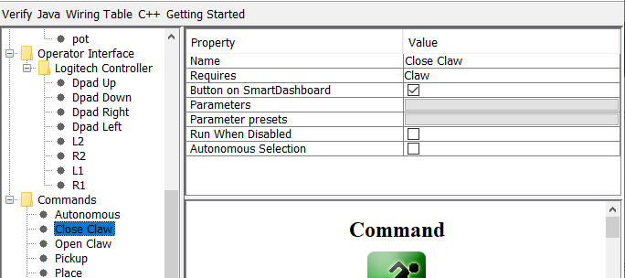
This is the definition of the CloseClaw command in RobotBuilder. Notice that it requires the Claw subsystem. This is explained in the next step.
Generated CloseClaw Class
11 // ROBOTBUILDER TYPE: Command.
12
13 package frc.robot.commands;
14 import edu.wpi.first.wpilibj2.command.CommandBase;
15
16 // BEGIN AUTOGENERATED CODE, SOURCE=ROBOTBUILDER ID=IMPORTS
17 import frc.robot.subsystems.Claw;
18
19 // END AUTOGENERATED CODE, SOURCE=ROBOTBUILDER ID=IMPORTS
20
21 /**
22 *
23 */
24 public class CloseClaw extends CommandBase {
25
26 // BEGIN AUTOGENERATED CODE, SOURCE=ROBOTBUILDER ID=VARIABLE_DECLARATIONS
27 private final Claw m_claw;
28
29 // END AUTOGENERATED CODE, SOURCE=ROBOTBUILDER ID=VARIABLE_DECLARATIONS
30
31 // BEGIN AUTOGENERATED CODE, SOURCE=ROBOTBUILDER ID=CONSTRUCTORS
32
33
34 public CloseClaw(Claw subsystem) {
35
36
37 // END AUTOGENERATED CODE, SOURCE=ROBOTBUILDER ID=CONSTRUCTORS
38 // BEGIN AUTOGENERATED CODE, SOURCE=ROBOTBUILDER ID=VARIABLE_SETTING
39
40 // END AUTOGENERATED CODE, SOURCE=ROBOTBUILDER ID=VARIABLE_SETTING
41 // BEGIN AUTOGENERATED CODE, SOURCE=ROBOTBUILDER ID=REQUIRES
42
43 m_claw = subsystem;
44 addRequirements(m_claw);
45
46 // END AUTOGENERATED CODE, SOURCE=ROBOTBUILDER ID=REQUIRES
47 }
48
49 // Called when the command is initially scheduled.
50 @Override
51 public void initialize() {
52 m_claw.open(); // (1)
53 }
54
55 // Called every time the scheduler runs while the command is scheduled.
56 @Override
57 public void execute() {
58 }
59
60 // Called once the command ends or is interrupted.
61 @Override
62 public void end(boolean interrupted) {
63 m_claw.stop(); // (3)
64 }
65
66 // Returns true when the command should end.
67 @Override
68 public boolean isFinished() {
69 return m_claw.isGripping(); // (2)
70 }
71
72 @Override
73 public boolean runsWhenDisabled() {
74 // BEGIN AUTOGENERATED CODE, SOURCE=ROBOTBUILDER ID=DISABLED
75 return false;
76
77 // END AUTOGENERATED CODE, SOURCE=ROBOTBUILDER ID=DISABLED
78 }
79 }
11// ROBOTBUILDER TYPE: Command.
12
13// BEGIN AUTOGENERATED CODE, SOURCE=ROBOTBUILDER ID=CONSTRUCTOR
14
15#include "commands/CloseClaw.h"
16
17CloseClaw::CloseClaw(Claw* m_claw)
18:m_claw(m_claw){
19
20 // Use AddRequirements() here to declare subsystem dependencies
21 // eg. AddRequirements(m_Subsystem);
22 SetName("CloseClaw");
23 AddRequirements({m_claw});
24
25// END AUTOGENERATED CODE, SOURCE=ROBOTBUILDER ID=CONSTRUCTOR
26
27}
28
29// Called just before this Command runs the first time
30void CloseClaw::Initialize() {
31 m_claw->Close(); // (1)
32}
33
34// Called repeatedly when this Command is scheduled to run
35void CloseClaw::Execute() {
36
37}
38
39// Make this return true when this Command no longer needs to run execute()
40bool CloseClaw::IsFinished() {
41 return m_claw->IsGripping(); // (2)
42}
43
44// Called once after isFinished returns true
45void CloseClaw::End(bool interrupted) {
46 m_claw->Stop(); // (3)
47}
48
49bool CloseClaw::RunsWhenDisabled() const {
50 // BEGIN AUTOGENERATED CODE, SOURCE=ROBOTBUILDER ID=DISABLED
51 return false;
52
53 // END AUTOGENERATED CODE, SOURCE=ROBOTBUILDER ID=DISABLED
54}
RobotBuilder will generate the class files for the CloseClaw command. The command represents the behavior of the claw, that is the operation over time. To operate this very simple claw mechanism the motor needs to operate in the close direction,. The Claw subsystem has methods to start the motor running in the right direction and to stop it. The commands responsibility is to run the motor for the correct time. The lines of code that are shown in the boxes are added to add this behavior.
Start the claw motor moving in the closing direction by calling the
Close()method that was added to the Claw subsystem in the CloseClaw Initialize method.This command is finished when the the limit switch in the Claw subsystem is tripped.
The
End()method is called when the command is finished and is a place to clean up. In this case, the motor is stopped since the time has run out.
Driving the Robot with Tank Drive and Joysticks
A common use case is to have a joystick that should drive some actuators that are part of a subsystem. The problem is that the joystick is created in the RobotContainer class and the motors to be controlled are in the subsystem. The idea is to create a command that, when scheduled, reads input from the joystick and calls a method that is created on the subsystem that drives the motors.
In this example a drive base subsystem is shown that is operated in tank drive using a pair of joysticks.
Create a Drive Train Subsystem
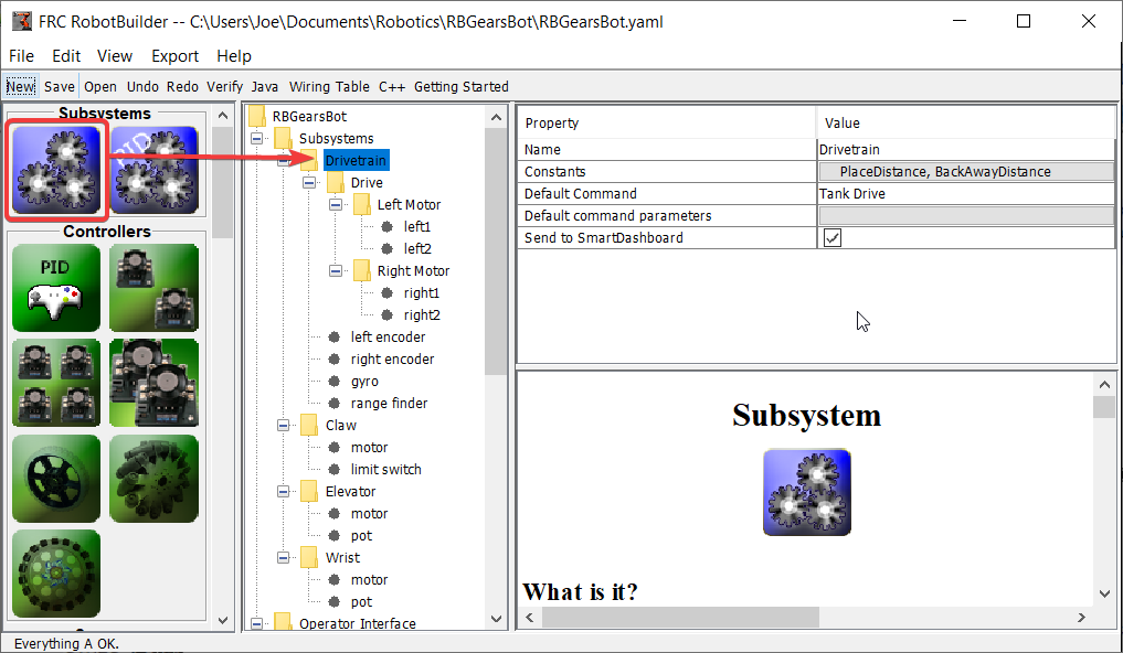
Create a subsystem called Drive Train. Its responsibility will be to handle the driving for the robot base.
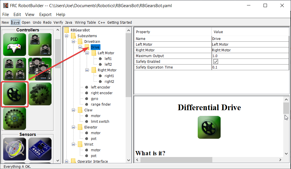
Inside the Drive Train create a Differential Drive object for a two motor drive. There is a left motor and right motor as part of the Differential Drive class.
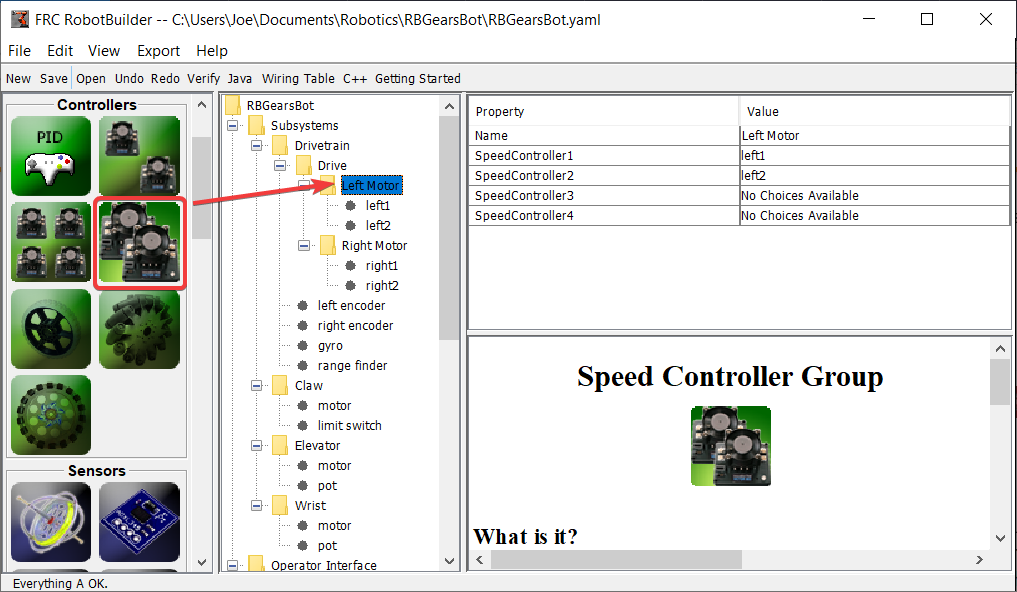
Since we want to use more then two motors to drive the robot, inside the Differential Drive, create two Motor Controller Groups. These will group multiple motor controllers so they can be used with Differential Drive.
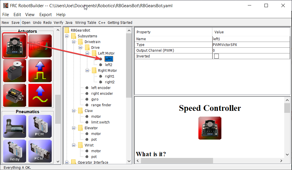
Finally, create two Motor Controllers in each Motor Controller Group.
Add the Joysticks to the Operator Interface
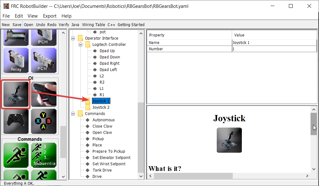
Add two joysticks to the Operator Interface, one is the left stick and the other is the right stick. The y-axis on the two joysticks are used to drive the robots left and right sides.
Note
Be sure to export your program to C++ or Java before continuing to the next step.
Create a Method to Write the Motors on the Subsystem
11// ROBOTBUILDER TYPE: Subsystem.
12
13package frc.robot.subsystems;
14
15
16import frc.robot.commands.*;
17import edu.wpi.first.wpilibj.livewindow.LiveWindow;
18import edu.wpi.first.wpilibj2.command.SubsystemBase;
19
20// BEGIN AUTOGENERATED CODE, SOURCE=ROBOTBUILDER ID=IMPORTS
21import edu.wpi.first.wpilibj.AnalogGyro;
22import edu.wpi.first.wpilibj.AnalogInput;
23import edu.wpi.first.wpilibj.CounterBase.EncodingType;
24import edu.wpi.first.wpilibj.Encoder;
25import edu.wpi.first.wpilibj.drive.DifferentialDrive;
26import edu.wpi.first.wpilibj.motorcontrol.MotorController;
27import edu.wpi.first.wpilibj.motorcontrol.MotorControllerGroup;
28import edu.wpi.first.wpilibj.motorcontrol.PWMVictorSPX;
29
30 // END AUTOGENERATED CODE, SOURCE=ROBOTBUILDER ID=IMPORTS
31
32
33/**
34 *
35 */
36public class Drivetrain extends SubsystemBase {
37 // BEGIN AUTOGENERATED CODE, SOURCE=ROBOTBUILDER ID=CONSTANTS
38public static final double PlaceDistance = 0.1;
39public static final double BackAwayDistance = 0.6;
40
41 // END AUTOGENERATED CODE, SOURCE=ROBOTBUILDER ID=CONSTANTS
42
43 // BEGIN AUTOGENERATED CODE, SOURCE=ROBOTBUILDER ID=DECLARATIONS
44private PWMVictorSPX left1;
45private PWMVictorSPX left2;
46private MotorControllerGroup leftMotor;
47private PWMVictorSPX right1;
48private PWMVictorSPX right2;
49private MotorControllerGroup rightMotor;
50private DifferentialDrive drive;
51private Encoder leftencoder;
52private Encoder rightencoder;
53private AnalogGyro gyro;
54private AnalogInput rangefinder;
55
56 // END AUTOGENERATED CODE, SOURCE=ROBOTBUILDER ID=DECLARATIONS
57
58 /**
59 *
60 */
61 public Drivetrain() {
62 // BEGIN AUTOGENERATED CODE, SOURCE=ROBOTBUILDER ID=CONSTRUCTORS
63left1 = new PWMVictorSPX(0);
64 addChild("left1",left1);
65 left1.setInverted(false);
66
67left2 = new PWMVictorSPX(1);
68 addChild("left2",left2);
69 left2.setInverted(false);
70
71leftMotor = new MotorControllerGroup(left1, left2 );
72 addChild("Left Motor",leftMotor);
73
74
75right1 = new PWMVictorSPX(5);
76 addChild("right1",right1);
77 right1.setInverted(false);
78
79right2 = new PWMVictorSPX(6);
80 addChild("right2",right2);
81 right2.setInverted(false);
82
83rightMotor = new MotorControllerGroup(right1, right2 );
84 addChild("Right Motor",rightMotor);
85
86
87drive = new DifferentialDrive(leftMotor, rightMotor);
88 addChild("Drive",drive);
89 drive.setSafetyEnabled(true);
90drive.setExpiration(0.1);
91drive.setMaxOutput(1.0);
92
93
94leftencoder = new Encoder(0, 1, false, EncodingType.k4X);
95 addChild("left encoder",leftencoder);
96 leftencoder.setDistancePerPulse(1.0);
97
98rightencoder = new Encoder(2, 3, false, EncodingType.k4X);
99 addChild("right encoder",rightencoder);
100 rightencoder.setDistancePerPulse(1.0);
101
102gyro = new AnalogGyro(0);
103 addChild("gyro",gyro);
104 gyro.setSensitivity(0.007);
105
106rangefinder = new AnalogInput(1);
107 addChild("range finder", rangefinder);
108
109
110
111 // END AUTOGENERATED CODE, SOURCE=ROBOTBUILDER ID=CONSTRUCTORS
112 }
113
114 @Override
115 public void periodic() {
116 // This method will be called once per scheduler run
117
118 }
119
120 @Override
121 public void simulationPeriodic() {
122 // This method will be called once per scheduler run when in simulation
123
124 }
125
126 // Put methods for controlling this subsystem
127 // here. Call these from Commands.
128
129 public void drive(double left, double right) {
130 drive.tankDrive(left, right);
131 }
132}
11// ROBOTBUILDER TYPE: Subsystem.
12#pragma once
13
14// BEGIN AUTOGENERATED CODE, SOURCE=ROBOTBUILDER ID=INCLUDES
15#include <frc2/command/SubsystemBase.h>
16#include <frc/AnalogGyro.h>
17#include <frc/AnalogInput.h>
18#include <frc/Encoder.h>
19#include <frc/drive/DifferentialDrive.h>
20#include <frc/motorcontrol/MotorControllerGroup.h>
21#include <frc/motorcontrol/PWMVictorSPX.h>
22
23// END AUTOGENERATED CODE, SOURCE=ROBOTBUILDER ID=INCLUDES
24
25/**
26 *
27 *
28 * @author ExampleAuthor
29 */
30class Drivetrain: public frc2::SubsystemBase {
31private:
32 // It's desirable that everything possible is private except
33 // for methods that implement subsystem capabilities
34 // BEGIN AUTOGENERATED CODE, SOURCE=ROBOTBUILDER ID=DECLARATIONS
35frc::AnalogInput m_rangefinder{1};
36frc::AnalogGyro m_gyro{0};
37frc::Encoder m_rightencoder{2, 3, false, frc::Encoder::k4X};
38frc::Encoder m_leftencoder{0, 1, false, frc::Encoder::k4X};
39frc::DifferentialDrive m_drive{m_leftMotor, m_rightMotor};
40frc::MotorControllerGroup m_rightMotor{m_right1, m_right2 };
41frc::PWMVictorSPX m_right2{6};
42frc::PWMVictorSPX m_right1{5};
43frc::MotorControllerGroup m_leftMotor{m_left1, m_left2 };
44frc::PWMVictorSPX m_left2{1};
45frc::PWMVictorSPX m_left1{0};
46
47 // END AUTOGENERATED CODE, SOURCE=ROBOTBUILDER ID=DECLARATIONS
48public:
49Drivetrain();
50
51 void Periodic() override;
52 void SimulationPeriodic() override;
53 void Drive(double left, double right);
54 // BEGIN AUTOGENERATED CODE, SOURCE=ROBOTBUILDER ID=CMDPIDGETTERS
55
56 // END AUTOGENERATED CODE, SOURCE=ROBOTBUILDER ID=CMDPIDGETTERS
57 // BEGIN AUTOGENERATED CODE, SOURCE=ROBOTBUILDER ID=CONSTANTS
58static constexpr const double PlaceDistance = 0.1;
59static constexpr const double BackAwayDistance = 0.6;
60
61 // END AUTOGENERATED CODE, SOURCE=ROBOTBUILDER ID=CONSTANTS
62
63
64};
11// ROBOTBUILDER TYPE: Subsystem.
12
13// BEGIN AUTOGENERATED CODE, SOURCE=ROBOTBUILDER ID=INCLUDES
14#include "subsystems/Drivetrain.h"
15#include <frc/smartdashboard/SmartDashboard.h>
16
17// END AUTOGENERATED CODE, SOURCE=ROBOTBUILDER ID=INCLUDES
18
19Drivetrain::Drivetrain(){
20 SetName("Drivetrain");
21 // BEGIN AUTOGENERATED CODE, SOURCE=ROBOTBUILDER ID=DECLARATIONS
22 SetSubsystem("Drivetrain");
23
24 AddChild("range finder", &m_rangefinder);
25
26
27 AddChild("gyro", &m_gyro);
28 m_gyro.SetSensitivity(0.007);
29
30 AddChild("right encoder", &m_rightencoder);
31 m_rightencoder.SetDistancePerPulse(1.0);
32
33 AddChild("left encoder", &m_leftencoder);
34 m_leftencoder.SetDistancePerPulse(1.0);
35
36 AddChild("Drive", &m_drive);
37 m_drive.SetSafetyEnabled(true);
38m_drive.SetExpiration(0.1_s);
39m_drive.SetMaxOutput(1.0);
40
41
42 AddChild("Right Motor", &m_rightMotor);
43
44
45 AddChild("right2", &m_right2);
46 m_right2.SetInverted(false);
47
48 AddChild("right1", &m_right1);
49 m_right1.SetInverted(false);
50
51 AddChild("Left Motor", &m_leftMotor);
52
53
54 AddChild("left2", &m_left2);
55 m_left2.SetInverted(false);
56
57 AddChild("left1", &m_left1);
58 m_left1.SetInverted(false);
59
60 // END AUTOGENERATED CODE, SOURCE=ROBOTBUILDER ID=DECLARATIONS
61}
62
63void Drivetrain::Periodic() {
64 // Put code here to be run every loop
65
66}
67
68void Drivetrain::SimulationPeriodic() {
69 // This method will be called once per scheduler run when in simulation
70
71}
72
73// BEGIN AUTOGENERATED CODE, SOURCE=ROBOTBUILDER ID=CMDPIDGETTERS
74
75// END AUTOGENERATED CODE, SOURCE=ROBOTBUILDER ID=CMDPIDGETTERS
76
77
78// Put methods for controlling this subsystem
79// here. Call these from Commands.
80
81 void Drivetrain::Drive(double left, double right) {
82 m_drive.TankDrive(left, right);
83 }
Create a method that takes the joystick inputs, in this case the the left and right driver joystick. The values are passed to the DifferentialDrive object that in turn does tank steering using the joystick values. Also create a method called stop() that stops the robot from driving, this might come in handy later.
Note
Some RobotBuilder output has been removed for this example for clarity
Read Joystick Values and Call the Subsystem Methods
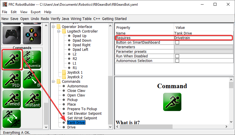
Create a command, in this case called Tank Drive. Its purpose will be to read the joystick values and send them to the Drive Base subsystem. Notice that this command Requires the Drive Train subsystem. This will cause it to stop running whenever anything else tries to use the Drive Train.
Note
Be sure to export your program to C++ or Java before continuing to the next step.
Add the Code to do the Driving
11// ROBOTBUILDER TYPE: Command.
12
13package frc.robot.commands;
14import edu.wpi.first.wpilibj.Joystick;
15import edu.wpi.first.wpilibj2.command.CommandBase;
16import frc.robot.RobotContainer;
17// BEGIN AUTOGENERATED CODE, SOURCE=ROBOTBUILDER ID=IMPORTS
18import frc.robot.subsystems.Drivetrain;
19
20 // END AUTOGENERATED CODE, SOURCE=ROBOTBUILDER ID=IMPORTS
21
22/**
23 *
24 */
25public class TankDrive extends CommandBase {
26
27 // BEGIN AUTOGENERATED CODE, SOURCE=ROBOTBUILDER ID=VARIABLE_DECLARATIONS
28 private final Drivetrain m_drivetrain;
29
30 // END AUTOGENERATED CODE, SOURCE=ROBOTBUILDER ID=VARIABLE_DECLARATIONS
31
32 private Joystick leftJoystick = RobotContainer.getInstance().getJoystick1();
33 private Joystick rightJoystick = RobotContainer.getInstance().getJoystick2();
34
35 // BEGIN AUTOGENERATED CODE, SOURCE=ROBOTBUILDER ID=CONSTRUCTORS
36
37
38 public TankDrive(Drivetrain subsystem) {
39
40
41 // END AUTOGENERATED CODE, SOURCE=ROBOTBUILDER ID=CONSTRUCTORS
42 // BEGIN AUTOGENERATED CODE, SOURCE=ROBOTBUILDER ID=VARIABLE_SETTING
43
44 // END AUTOGENERATED CODE, SOURCE=ROBOTBUILDER ID=VARIABLE_SETTING
45 // BEGIN AUTOGENERATED CODE, SOURCE=ROBOTBUILDER ID=REQUIRES
46
47 m_drivetrain = subsystem;
48 addRequirements(m_drivetrain);
49
50 // END AUTOGENERATED CODE, SOURCE=ROBOTBUILDER ID=REQUIRES
51 }
52
53 // Called when the command is initially scheduled.
54 @Override
55 public void initialize() {
56 }
57
58 // Called every time the scheduler runs while the command is scheduled.
59 @Override
60 public void execute() {
61 m_drivetrain.drive(leftJoystick.getY(), rightJoystick.getY());
62 }
63
64 // Called once the command ends or is interrupted.
65 @Override
66 public void end(boolean interrupted) {
67 m_drivetrain.drive(0.0, 0.0);
68 }
69
70 // Returns true when the command should end.
71 @Override
72 public boolean isFinished() {
73 return false;
74 }
75
76 @Override
77 public boolean runsWhenDisabled() {
78 // BEGIN AUTOGENERATED CODE, SOURCE=ROBOTBUILDER ID=DISABLED
79 return false;
80
81 // END AUTOGENERATED CODE, SOURCE=ROBOTBUILDER ID=DISABLED
82 }
83}
11// ROBOTBUILDER TYPE: Command.
12
13#pragma once
14
15 // BEGIN AUTOGENERATED CODE, SOURCE=ROBOTBUILDER ID=INCLUDES
16
17#include <frc2/command/CommandHelper.h>
18#include <frc2/command/CommandBase.h>
19
20#include "subsystems/Drivetrain.h"
21
22 // END AUTOGENERATED CODE, SOURCE=ROBOTBUILDER ID=INCLUDES
23#include "RobotContainer.h"
24#include <frc/Joystick.h>
25
26/**
27 *
28 *
29 * @author ExampleAuthor
30 */
31class TankDrive: public frc2::CommandHelper<frc2::CommandBase, TankDrive> {
32public:
33 // BEGIN AUTOGENERATED CODE, SOURCE=ROBOTBUILDER ID=CONSTRUCTOR
34 explicit TankDrive(Drivetrain* m_drivetrain);
35
36 // END AUTOGENERATED CODE, SOURCE=ROBOTBUILDER ID=CONSTRUCTOR
37
38void Initialize() override;
39void Execute() override;
40bool IsFinished() override;
41void End(bool interrupted) override;
42bool RunsWhenDisabled() const override;
43
44
45private:
46 // BEGIN AUTOGENERATED CODE, SOURCE=ROBOTBUILDER ID=VARIABLES
47
48
49Drivetrain* m_drivetrain;
50frc::Joystick* m_leftJoystick;
51frc::Joystick* m_rightJoystick;
52
53 // END AUTOGENERATED CODE, SOURCE=ROBOTBUILDER ID=VARIABLES
54};
11// ROBOTBUILDER TYPE: Command.
12
13// BEGIN AUTOGENERATED CODE, SOURCE=ROBOTBUILDER ID=CONSTRUCTOR
14
15#include "commands/TankDrive.h"
16
17TankDrive::TankDrive(Drivetrain* m_drivetrain)
18:m_drivetrain(m_drivetrain){
19
20 // Use AddRequirements() here to declare subsystem dependencies
21 // eg. AddRequirements(m_Subsystem);
22 SetName("TankDrive");
23 AddRequirements({m_drivetrain});
24
25// END AUTOGENERATED CODE, SOURCE=ROBOTBUILDER ID=CONSTRUCTOR
26 m_leftJoystick = RobotContainer::GetInstance()->getJoystick1();
27 m_rightJoystick = RobotContainer::GetInstance()->getJoystick2();
28}
29
30// Called just before this Command runs the first time
31void TankDrive::Initialize() {
32
33}
34
35// Called repeatedly when this Command is scheduled to run
36void TankDrive::Execute() {
37 m_drivetrain->Drive(m_leftJoystick->GetY(),m_rightJoystick->GetY());
38}
39
40// Make this return true when this Command no longer needs to run execute()
41bool TankDrive::IsFinished() {
42 return false;
43}
44
45// Called once after isFinished returns true
46void TankDrive::End(bool interrupted) {
47 m_drivetrain->Drive(0,0);
48}
49
50bool TankDrive::RunsWhenDisabled() const {
51 // BEGIN AUTOGENERATED CODE, SOURCE=ROBOTBUILDER ID=DISABLED
52 return false;
53
54 // END AUTOGENERATED CODE, SOURCE=ROBOTBUILDER ID=DISABLED
55}
Add code to the execute method to do the actual driving. All that is needed is to get the Joystick objects for the left and right drive joysticks and pass them to the Drive Train subsystem. The subsystem just uses them for the tank steering method on its DifferentialDrive object. And we get tank steering.
We also filled in the end() method so that when this command is interrupted or stopped, the motors will be stopped as a safety precaution.
Make Default Command
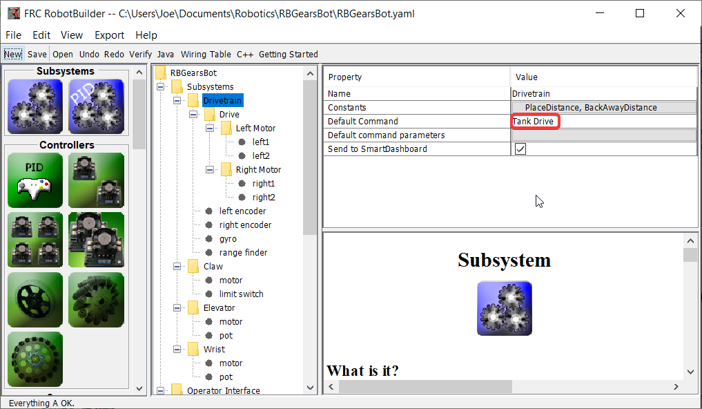
The last step is to make the Tank Drive command be the “Default Command” for the Drive Train subsystem. This means that whenever no other command is using the Drive Train, the Joysticks will be in control. This is probably the desirable behavior. When the autonomous code is running, it will also require the drive train and interrupt the Tank Drive command. When the autonomous code is finished, the DriveWithJoysticks command will restart automatically (because it is the default command), and the operators will be back in control. If you write any code that does teleop automatic driving, those commands should also “require” the DriveTrain so that they too will interrupt the Tank Drive command and have full control.
Note
Be sure to export your program to C++ or Java before continuing.
RobotBuilder - Advanced
Using PIDSubsystem to Control Actuators
More advanced subsystems will use sensors for feedback to get guaranteed results for operations like setting elevator heights or wrist angles. PIDSubsystems use feedback to control the actuator and drive it to a particular position. In this example we use an elevator with a 10-turn potentiometer connected to it to give feedback on the height. The PIDSubsystem has a built-in PIDController to automatically control the mechanism to the correct setpoints.
Create a PIDSubsystem
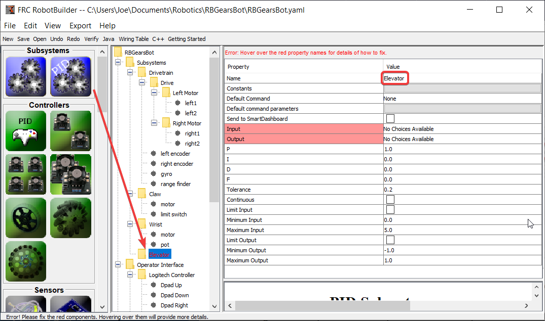
Creating a subsystem that uses feedback to control the position or speed of a mechanism is very easy.
Drag a PIDSubsystem from the palette to the Subsystems folder in the robot description
Rename the PID Subsystem to a more meaningful name for the subsystem, in this case Elevator
Notice that some of the parts of the robot description have turned red. This indicates that these components (the PIDSubsystem) haven’t been completed and need to be filled in. The properties that are either missing or incorrect are shown in red.
Adding Sensors and Actuators to the PIDSubsystem
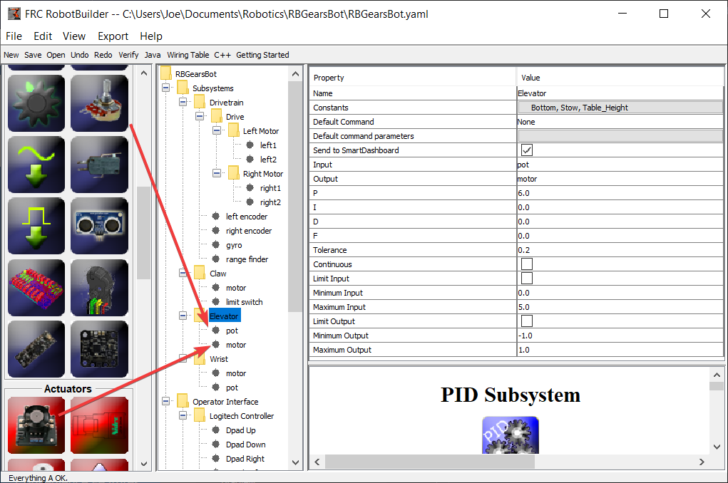
Add the missing components for the PIDSubsystem
Drag in the actuator (a motor controller) to the particular subsystem - in this case the Elevator
Drag the sensor that will be used for feedback to the subsystem, in this case the sensor is a potentiometer that might give elevator height feedback.
Fill in the PID Parameters
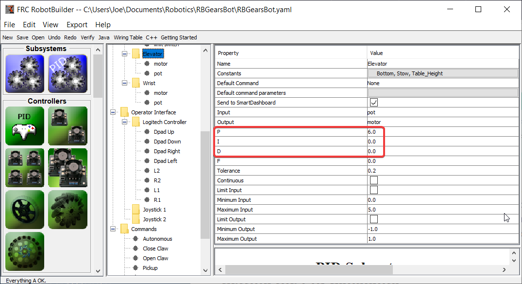
The P, I, and D values need to be filled in to get the desired sensitivity and stability of the component. In the case of our elevator we use a proportional constant of 6.0 and 0 for the I and D terms.
Create Setpoint Constants
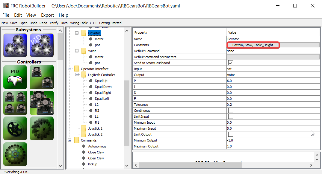
In order to make it easier to manage elevator setpoints, we will create constants to manage the setpoints. Click on the constants box to bring up the constants dialog.
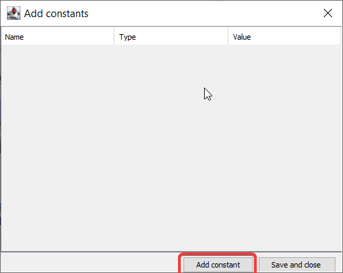
Click on the add constant button
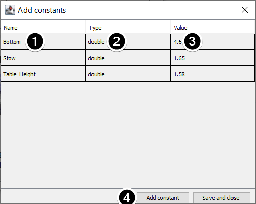
Fill in a name for the constant, in this case: Bottom
Select a type for the constant from the drop-down menu, in this case: double
Select a value for the constant, in this case: 4.65
Click add constant to continue adding constants
After entering all constants, Click Save and close
Writing the Code for a PIDSubsystem
The skeleton of the PIDSubsystem is generated by the RobotBuilder and we have to fill in the rest of the code to provide the potentiometer value and drive the motor with the output of the embedded PIDController.
Make sure the Elevator PID subsystem has been created in the RobotBuilder. Once it’s all set, generate Java/C++ code for the project using the Export menu or the Java/C++ toolbar menu.
RobotBuilder generates the PIDSubsystem methods such that no additional code is needed for basic operation.
Setting the PID Constants
The height constants and PID constants are automatically generated.
public class Elevator extends PIDSubsystem {
// BEGIN AUTOGENERATED CODE, SOURCE=ROBOTBUILDER ID=CONSTANTS
public static final double Bottom = 4.6;
public static final double Stow = 1.65;
public static final double Table_Height = 1.58;
// END AUTOGENERATED CODE, SOURCE=ROBOTBUILDER ID=CONSTANTS
// BEGIN AUTOGENERATED CODE, SOURCE=ROBOTBUILDER ID=DECLARATIONS
private AnalogPotentiometer pot;private PWMVictorSPX motor;
//P I D Variables
private static final double kP = 6.0;
private static final double kI = 0.0;
private static final double kD = 0.0;
private static final double kF = 0.0;
// END AUTOGENERATED CODE, SOURCE=ROBOTBUILDER ID=DECLARATIONS
// BEGIN AUTOGENERATED CODE, SOURCE=ROBOTBUILDER ID=CONSTANTS
static constexpr const double Bottom = 4.6;
static constexpr const double Stow = 1.65;
static constexpr const double Table_Height = 1.58;
static constexpr const double kP = 6.0;
static constexpr const double kI = 0.0;
static constexpr const double kD = 0.0;
static constexpr const double kF = 0.0;
// END AUTOGENERATED CODE, SOURCE=ROBOTBUILDER ID=CONSTANTS
Get Potentiometer Measurement
@Override
public double getMeasurement() {
// BEGIN AUTOGENERATED CODE, SOURCE=ROBOTBUILDER ID=SOURCE
return pot.get();
// END AUTOGENERATED CODE, SOURCE=ROBOTBUILDER ID=SOURCE
}
double Elevator::GetMeasurement() {
// BEGIN AUTOGENERATED CODE, SOURCE=ROBOTBUILDER ID=SOURCE
return m_pot.Get();
// END AUTOGENERATED CODE, SOURCE=ROBOTBUILDER ID=SOURCE
}
The getMeasurement() method is used to set the value of the sensor that is providing the feedback for the PID controller. In this case, the code is automatically generated and returns the potentiometer voltage as returned by the get() method.
Calculate PID Output
@Override
public void useOutput(double output, double setpoint) {
output += setpoint*kF;
// BEGIN AUTOGENERATED CODE, SOURCE=ROBOTBUILDER ID=OUTPUT
motor.set(output);
// END AUTOGENERATED CODE, SOURCE=ROBOTBUILDER ID=OUTPUT
}
void Elevator::UseOutput(double output, double setpoint) {
output += setpoint*kF;
// BEGIN AUTOGENERATED CODE, SOURCE=ROBOTBUILDER ID=OUTPUT
m_motor.Set(output);
// END AUTOGENERATED CODE, SOURCE=ROBOTBUILDER ID=OUTPUT
}
The useOutput method writes the calculated PID output directly to the motor.
That’s all that is required to create the Elevator PIDSubsystem.
Setpoint Command
A Setpoint Command works in conjunction with a PIDSubsystem to drive an actuator to a particular angle or position that is measured using a potentiometer or encoder. This happens so often that there is a shortcut in RobotBuilder to do this task.
Start with a PIDSubsystem
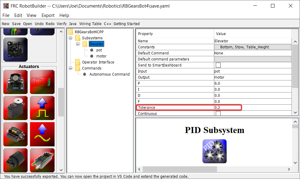
Suppose in a robot there is a wrist joint with a potentiometer that measures the angle. First create a PIDSubsystem that include the motor that moves the wrist joint and the potentiometer that measures the angle. The PIDSubsystem should have all the PID constants filled in and working properly.
It is important to set the Tolerance parameter. This controls how far off the current value can be from the setpoint and be considered on target. This is the criteria that the SetpointCommand uses to move onto the next command.
Creating the Setpoint Command
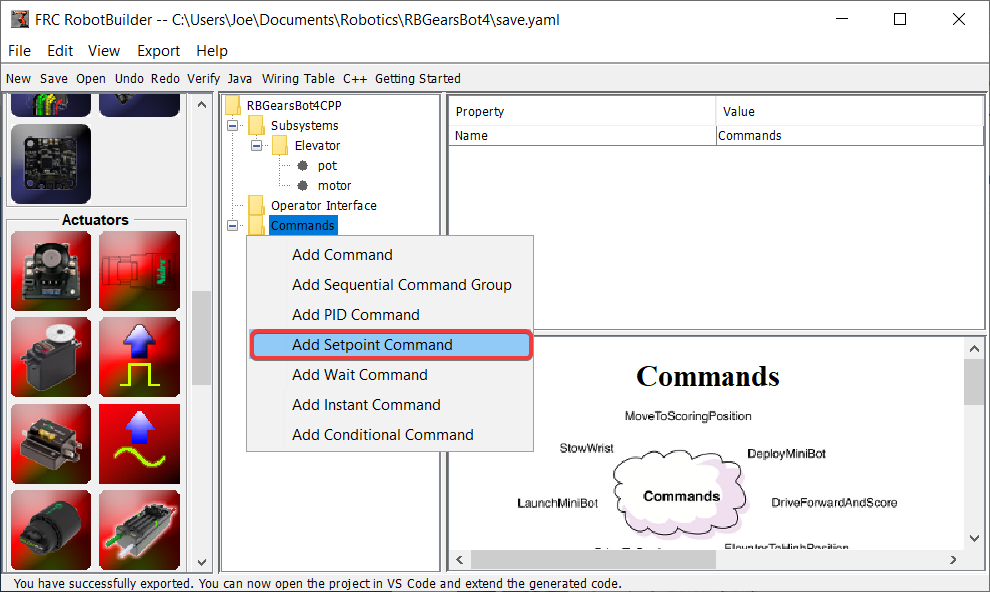
Right-click on the Commands folder in the palette and select “Add Setpoint command”.
Setpoint Command Parameters
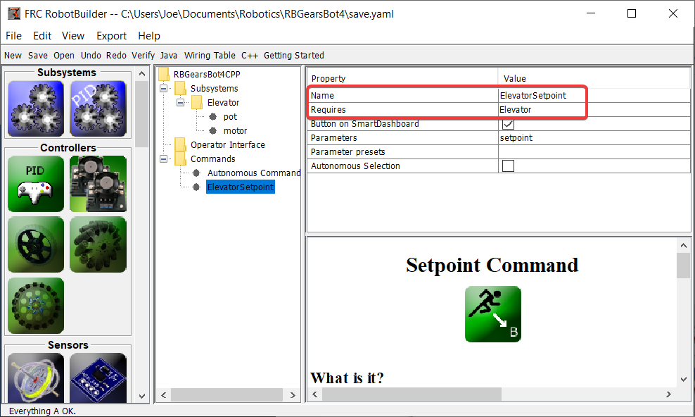
Fill in the name of the new command. The Requires field is the PIDSubsystem that is being driven to a setpoint, in this case the Elevator subsystem.
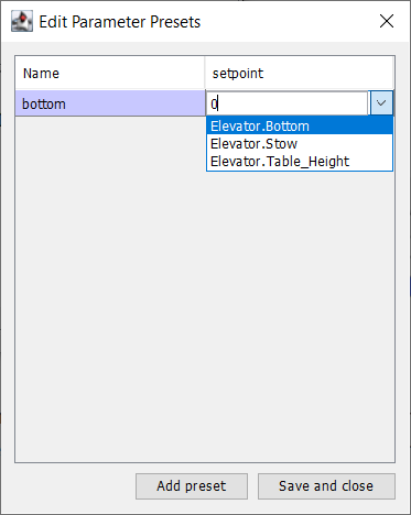
Click on the Parameter Presets to set up the setpoints.
Select Add Preset
Enter a preset name (in this case ‘bottom’
Click the dropdown next to the setpoint entry box
Select the Elevator.Bottom constant, that was created in the Elevator subystem previously
Repeat steps 2-5 for the other setpoints.
Click Save and close
There is no need to fill in any code for this command, it is automatically created by RobotBuilder.
Whenever this command is scheduled, it will automatically drive the subsystem to the specified setpoint. When the setpoint is reached within the tolerance specified in the PIDSubsystem, the command ends and the next command starts. It is important to specify a tolerance in the PIDSubsystem or this command might never end because the tolerance is not achieved.
Note
For more information about PID Control, please see the Advanced Controls Introduction.
Adding Custom Components
RobotBuilder works very well for creating robot programs that just use WPILib for motors, controllers, and sensors. But for teams that use custom classes, RobotBuilder doesn’t have any support for those classes, so a few steps need to be taken to use them in RobotBuilder
Custom Component Structure
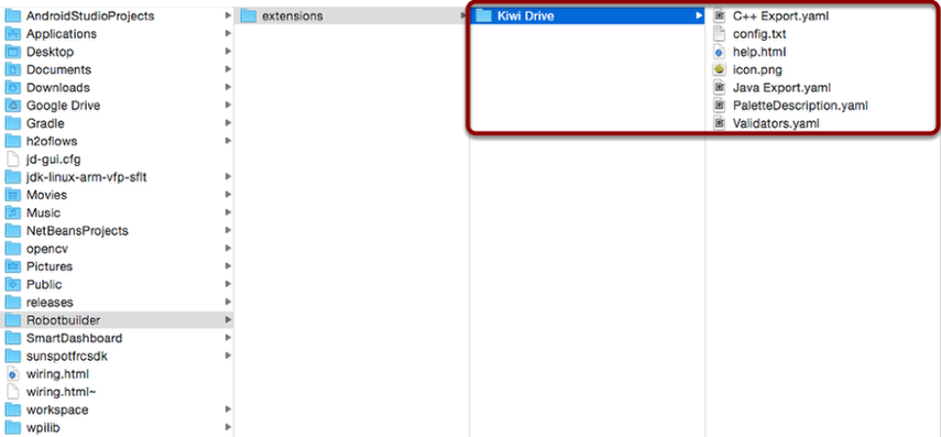
Custom components all go in ~/wpilib/YYYY/Robotbuilder/extensions where ~ is C:\Users\Public on Windows and YYYY is the FRC® year.
There are seven files and one folder that are needed for a custom component. The folder contains the files describing the component and how to export it. It should have the same name as the component (e.g.”Kiwi Drive” for a kiwi drive controller, “Robot Drive 6” for a six-motor drive controller, etc.). The files should have the same names and extensions as the ones shown here. Other files can be in the folder along with these seven, but the seven must be present for RobotBuilder to recognize the custom component.
PaletteDescription.yaml
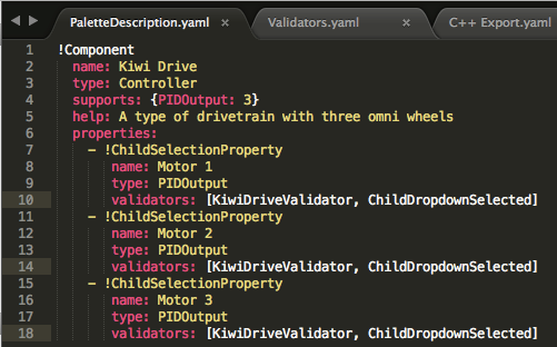
Line-by-line:
!Component: Declares the beginning of a new component
name: The name of the component. This is what will show up in the palette/tree – this should also be the same as the name of the containing folder
type: the type of the component (these will be explained in depth later on)
supports: a map of the amount of each type of component this can support. Motor controllers in RobotBuilder are all PIDOutputs, so a kiwi drive can support three PIDOutputs. If a component doesn’t support anything (such as sensors or motor controllers), just leave this line out
help: a short string that gives a helpful message when one of these components is hovered over
properties: a list of the properties of this component. In this kiwi drive example, there are three very similar properties, one for each motor. A ChildSelectionProperty allows the user to choose a component of the given type from the subcomponents of the one being edited (so here, they would show a dropdown asking for a PIDOutput - i.e. a motor controller - that has been added to the kiwi drive)
The types of component RobotBuilder supports (these are case-sensitive):
Command
Subsystem
PIDOutput (motor controller)
PIDSource (sensor that implements PIDSource e.g. analog potentiometer, encoder)
Sensor (sensor that does not implement PIDSource e.g. limit switch)
Controller (robot drive, PID controller, etc.)
Actuator (an output that is not a motor, e.g. solenoid, servo)
Joystick
Joystick Button
Properties
The properties relevant for a custom component:
StringProperty: used when a component needs a string e.g. the name of the component
BooleanProperty: used when a component needs a boolean value e.g. putting a button on the SmartDashboard
DoubleProperty: used when a component needs a number value e.g. PID constantsChoicesProperty
ChildSelectionProperty: used when you need to choose a child component e.g. motor controllers in a RobotDrive
TypeSelectionProperty: used when you need to choose any component of the given type from anywhere in the program e.g. input and output for a PID command
The fields for each property are described below:
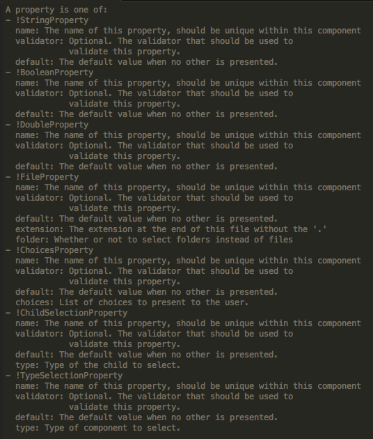
Validators.yaml
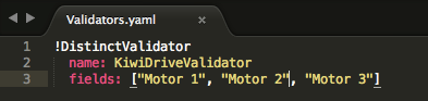
You may have noticed “KiwiDriveValidator” in the validators entry of each of the motor properties in PaletteDescription.yaml. It’s not a built-in validator, so it had to be defined in Validators.yaml. This example validator is very simple - it just makes sure that each of the named fields has a different value than the others.
Built-in Validators and Validator Types
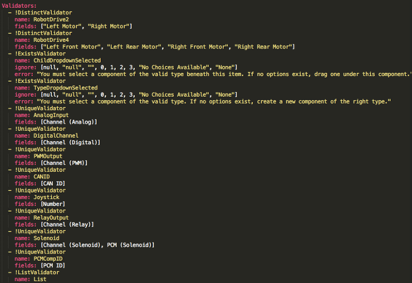
The built-in validators are very useful (especially the UniqueValidators for port/channel use), but sometimes a custom validator is needed, like in the previous step
DistinctValidator: Makes sure the values of each of the given fields are unique
ExistsValidator: Makes sure that a value has been set for the property using this validator
UniqueValidator: Makes sure that the value for the property is unique globally for the given fields
ListValidator: Makes sure that all the values in a list property are valid
C++ Export.yaml
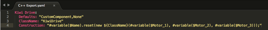
A line-by-line breakdown of the file:
Kiwi Drive: the name of the component being exported. This is the same as the name set in PaletteDescription.yaml, and the name of the folder containing this file
Defaults: provides some default values for includes needed by this component, the name of the class, a construction template, and more. The CustomComponent default adds an include for
Custom/${ClassName}.hto every generated file that uses the component (e.g.RobotDrive.hwould have#include "Custom/KiwiDrive.hthe top of the file)ClassName: the name of the custom class you’re adding.
Construction: an instruction for how the component should be constructed. Variables will be replaced with their values (“${ClassName}” will be replaced with “KiwiDrive”), then macros will be evaluated (for example,
#variable($Name)may be replaced withdrivebaseKiwiDrive).
This example expects a KiwiDrive class with the constructor
KiwiDrive(SpeedController, SpeedController, SpeedController)
If your team uses Java, this file can be empty.
Java Export.yaml
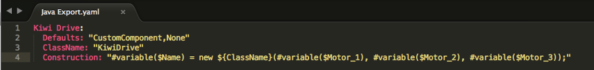
Very similar to the C++ export file; the only difference should be the Construction line. This example expects a KiwiDrive class with the constructor
KiwiDrive(SpeedController, SpeedController, SpeedController)
If your team uses C++, this file can be empty.
Using Macros and Variables
Macros are simple functions that RobotBuilder uses to turn variables into text that will be inserted into generated code. They always start with the “#” symbol, and have a syntax similar to functions: <macro_name>( arg0, arg1, arg2, ...). The only macro you’ll probably need to use is #variable( component_name )
#variable takes a string, usually the a variable defined somewhere (i.e. “Name” is the name given to the component in RobotBuilder, such as “Arm Motor”), and turns it into the name of a variable defined in the generated code. For example, #variable("Arm Motor") results in the string ArmMotor
Variables are referenced by placing a dollar sign (“$”) in front of the variable name, which an optionally be placed inside curly braces to easily distinguish the variable from other text in the file. When the file is parsed, the dollar sign, variable name, and curly braces are replaced with the value of the variable (e.g. ${ClassName} is replaced with KiwiDrive).
Variables are either component properties (e.g. “Motor 1”, “Motor 2”, “Motor 3” in the kiwi drive example), or one of the following:
Short_Name: the name given to the component in the editor panel in RobotBuilder
Name: the full name of the component. If the component is in a subsystem, this will be the short name appended to the name of the subsystem
Export: The name of the file this component should be created in, if any. This should be “RobotMap” for components like actuators, controllers, and sensors; or “OI” for things like gamepads or other custom OI components. Note that the “CustomComponent” default will export to the RobotMap.
Import: Files that need to be included or imported for this component to be able to be used.
Declaration: an instruction, similar to Construction, for how to declare a variable of this component type. This is taken care of by the default “None”
Construction: an instruction for how to create a new instance of this component
LiveWindow: an instruction for how to add this component to the LiveWindow
Extra: instructions for any extra functions or method calls for this component to behave correctly, such as encoders needing to set the encoding type.
Prototype (C++ only): The prototype for a function to be created in the file the component is declared in, typically a getter in the OI class
Function: A function to be created in the file the component is declared in, typically a getter in the OI class
PID: An instruction for how to get the PID output of the component, if it has one (e.g.
#variable($Short_Name)->PIDGet())ClassName: The name of the class that the component represents (e.g.
KiwiDriveorJoystick)
If you have variables with spaces in the name (such as “Motor 1”, “Right Front Motor”, etc.), the spaces need to be replaced with underscores when using them in the export files.
help.html
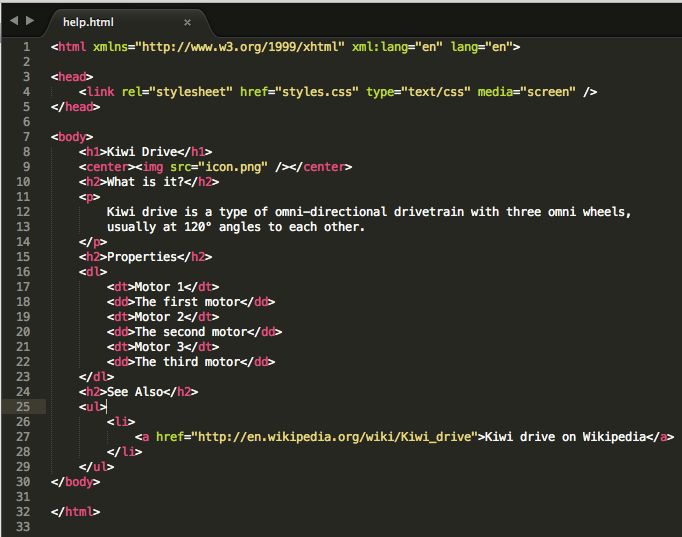
A HTML file giving information on the component. It is better to have this be as detailed as possible, though it certainly isn’t necessary if the programmer(s) are familiar enough with the component, or if it’s so simple that there’s little point in a detailed description.
config.txt
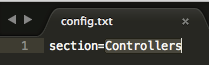
A configuration file to hold miscellaneous information about the component. Currently, this only has the section of the palette to put the component in.
The sections of the palette (these are case sensitive):
Subsystems
Controllers
Sensors
Actuators
Pneumatics
OI
Commands
icon.png
The icon that shows up in the palette and the help page. This should be a 64x64 .png file.
It should use the color scheme and general style of the section it’s in to avoid visual clutter, but this is entirely optional. Photoshop .psd files of the icons and backgrounds are in src/main/icons/icons and png files of the icons and backgrounds are in src/main/resources/icons.
Robot Simulation
Introduction to Robot Simulation
Often a team may want to test their code without having an actual robot available. WPILib provides teams with the ability to simulate various robot features using simple gradle commands.
Enabling Desktop Support
Use of the Desktop Simulator requires Desktop Support to be enabled. This can be done by checking the “Enable Desktop Support Checkbox” when creating your robot project or by running “WPILib: Change Desktop Support Enabled Setting” from the Visual Studio Code command palette.
Desktop support can also be enabled by manually editing your build.gradle file located at the root of your robot project. Simply change includeDesktopSupport = false to includeDesktopSupport = true
def includeDesktopSupport = true
Important
It is important to note that enabling desktop/simulation support can have unintended consequences. Not all vendors will support this option, and code that uses their libraries may even crash when attempting to run simulation!
If at any point in time you want to disable Desktop Support, simply re-run the “WPILib: Change Desktop Support Enabled Setting” from the command palette.
Additional C++ Dependency
C++ robot simulation requires that a native compiler to be installed. For Windows, this would be Visual Studio 2022 or 2019 (not VS Code), macOS requires Xcode, and Linux (Ubuntu) requires the build-essential package.
Ensure the Desktop Development with C++ option is checked in the Visual Studio installer for simulation support.
Running Robot Simulation
Basic robot simulation can be run using VS Code. This can be done without using any commands by using VS Code’s command palette.
Your console output in Visual Studio Code should look like the below. However, teams probably will want to actually test their code versus just running the simulation. This can be done using WPILib’s Simulation GUI.
********** Robot program starting **********
Default disabledInit() method... Override me!
Default disabledPeriodic() method... Override me!
Default robotPeriodic() method... Override me!
Important
Simulation can also be run outside of VS Code using ./gradlew simulateJava for Java or ./gradlew simulateNative for C++.
Running Robot Dashboards
Both Shuffleboard and SmartDashboard can be used with WPILib simulation.
Shuffleboard
Shuffleboard is automatically configured to look for a NetworkTables instance from the robotRIO but not from other sources. To connect to Shuffleboard, open Shuffleboard preferences from the File menu and select NetworkTables under Plugins on the left navigation bar. In the Server field, type in the IP address or hostname of the NetworkTables host. For a standard simulation configuration, use localhost.
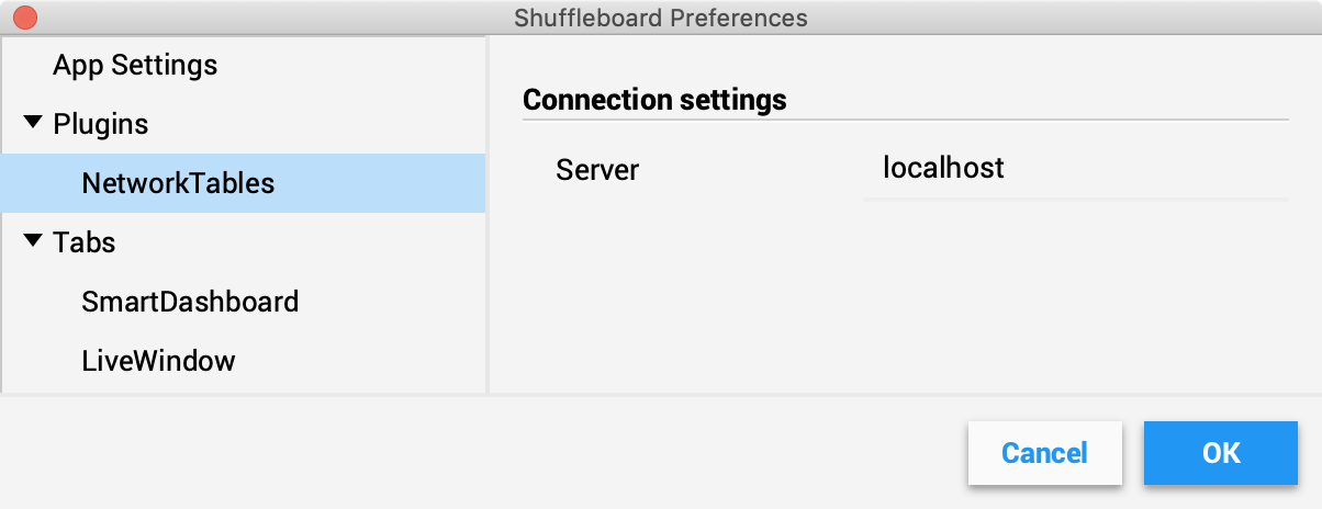
SmartDashboard
SmartDashboard is automatically configured to look for a NetworkTables instance from the roboRIO, but not from other sources. To connect to SmartDashboard, open SmartDashboard preferences under the File menu and in the Team Number field, enter the IP address or hostname of the NetworkTables host. For a standard simulation configuration, use localhost.
Simulation Specific User Interface Elements
WPILib has extended robot simulation to introduce a graphical user interface (GUI) component. This allows teams to easily visualize their robot’s inputs and outputs.
Note
The Simulation GUI is very similar in many ways to Glass. Some of the following pages will link to Glass sections that describe elements common to both GUIs.
Running the GUI
You can simply launch the GUI via the Run Simulation command palette option.
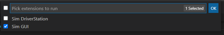
And the Sim GUI option should popup in a new dialog and will be selected by default. Press Ok. This will now launch the Simulation GUI!
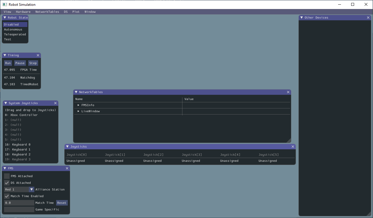
Using the GUI
Learning the Layout
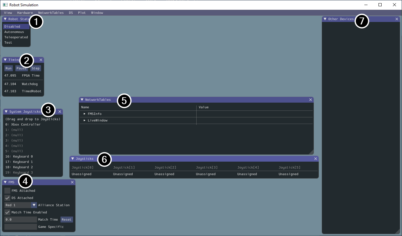
The following items are shown on the simulation GUI by default:
Robot State - This is the robot’s current state or “mode”. You can click on the labels to change mode as you would on the normal Driver Station.
Timing - Shows the values of the Robot’s timers and allows the timing to be manipulated.
System Joysticks - This is a list of joysticks connected to your system currently.
FMS - This is used for simulating many of the common FMS systems.
NetworkTables - This shows the data that has been published to NetworkTables.
Joysticks - This is joysticks that the robot code can directly pull from.
Other Devices - This includes devices that do not fall into any of the other categories, such as the ADXRS450 gyro that is included in the Kit of Parts or third party devices that support simulation.
The following items can be added from the Hardware menu, but are not shown by default.
Addressable LEDs - This shows LEDs controlled by the
AddressableLEDClass.Analog Inputs - This includes any devices that would normally use the ANALOG IN connector on the roboRIO, such as any Analog based gyros.
DIO - (Digital Input Output) This includes any devices that use the DIO connector on the roboRIO.
Encoders - This will show any instantiated devices that extend or use the
Encoderclass.PDPs - This shows the Power Distribution Panel object.
PWM Outputs - This is a list of instantiated PWM devices. This will appear as many devices as you instantiate in robot code, as well as their outputs.
Relays - This includes any relay devices. This includes VEX Spike relays.
Solenoids - This is a list of “connected” solenoids. When you create a solenoid object and push outputs, these are shown here.
Adding a System Joystick to Joysticks
To add a joystick from the list of system joysticks, simply click and drag a shown joystick under the “System Joysticks” menu to the “Joysticks” menu”.
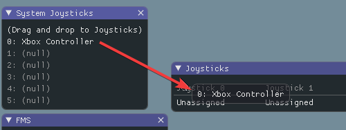
Note
The FRC® Driver Station does special mapping to gamepads connected and the WPILib simulator does not “map” these by default. You can turn on this behavior by pressing the “Map gamepad” toggle underneath the “Joysticks” menu.
Using the Keyboard as a Joystick
You add a keyboard to the list of system joysticks by clicking and dragging one of the keyboard items (e.g. Keyboard 0) just like a joystick above. To edit the settings of the keyboard go to the DS item in the menu bar then choose Keyboard 0 Settings. This allows you to control which keyboard buttons control which axis. This is a common example of how to make the keyboard similar to a split sticks arcade drive on an Xbox controller (uses axis 1 & 4):
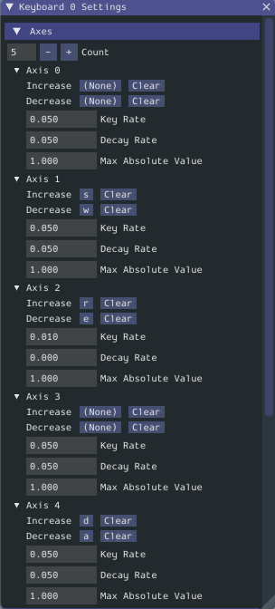
Modifying ADXRS450 Inputs
Using the ADXRS450 object is a fantastic way to test gyro based outputs. This will show up in the “Other Devices” menu. A drop down menu is then exposed that shows various options such as “Connected”, “Angle”, and “Rate”. All of these values are values that you can change, and that your robot code and use on-the-fly.
Determining Simulation from Robot Code
In cases where vendor libraries do not compile when running the robot simulation, you can wrap their content with RobotBase.isReal() which returns a boolean.
TalonSRX motorLeft;
TalonSRX motorRight;
public Robot() {
if (RobotBase.isReal()) {
motorLeft = new TalonSRX(0);
motorRight = new TalonSRX(1);
}
}
Note
Reassigning value types in C++ requires move or copy assignment; vendors classes that both do not support the SIM and lack a move or copy assignment operator cannot be worked around with conditional allocation unless a pointer is used, instead of a value type.
Changing View Settings
The View menu item contains Zoom and Style settings that can be customized. The Zoom option dictates the size of the text in the application whereas the Style option allows you to select between the Classic, Light, and Dark modes.
An example of the Dark style setting is below:
Clearing Application Data
Application data for the Simulation GUI, including widget sizes and positions as well as other custom information for widgets is stored in a imgui.ini file. This file is stored in the root of the project directory that the simulation is run from.
The imgui.ini configuration file can simply be deleted to restore the Simulation GUI to a “clean slate”.
Physics Simulation with WPILib
Because state-space notation allows us to compactly represent the dynamics of systems, we can leverage it to provide a backend for simulating physical systems on robots. The goal of these simulators is to simulate the motion of robot mechanisms without modifying existing non-simulation user code. The basic flow of such simulators is as follows:
In normal user code:
PID or similar control algorithms generate voltage commands from encoder (or other sensor) readings
Motor outputs are set
In simulation periodic code:
WPILib’s Simulation Classes
The following physics simulation classes are available in WPILib:
LinearSystemSim, for modeling systems with linear dynamics
FlywheelSim
DifferentialDrivetrainSim
ElevatorSim, which models gravity
SingleJointedArmSim, which models gravity
BatterySim, which simply estimates battery voltage sag based on drawn currents
All simulation classes (with the exception of the differential drive simulator) inherit from the LinearSystemSim class. By default, the dynamics are the linear system dynamics \(\mathbf{x}_{k+1} = \mathbf{A}\mathbf{x}_k + \mathbf{B}\mathbf{u}_k\). Subclasses override the UpdateX(x, u, dt) method to provide custom, nonlinear dynamics, such as modeling gravity.
Note
Swerve support for simulation is in the works, but we cannot provide an ETA. For updates on progress, please follow this pull request.
Usage in User Code
The following is available from the WPILib elevatorsimulation example project.
In addition to standard objects such as motors and encoders, we instantiate our elevator simulator using known constants such as carriage mass and gearing reduction. We also instantiate an EncoderSim, which sets the distance and rate read by our our Encoder.
In the following example, we simulate an elevator given the mass of the moving carriage (in kilograms), the radius of the drum driving the elevator (in meters), the gearing reduction between motor and drum as output over input (so usually greater than one), the minimum and maximum height of the elevator (in meters), and some random noise to add to our position estimate.
Note
The elevator and arm simulators will prevent the simulated position from exceeding given minimum or maximum heights or angles. If you wish to simulate a mechanism with infinite rotation or motion, LinearSystemSim may be a better option.
53 // Simulation classes help us simulate what's going on, including gravity.
54 private final ElevatorSim m_elevatorSim =
55 new ElevatorSim(
56 m_elevatorGearbox,
57 kElevatorGearing,
58 kCarriageMass,
59 kElevatorDrumRadius,
60 kMinElevatorHeight,
61 kMaxElevatorHeight,
62 VecBuilder.fill(0.01));
63 private final EncoderSim m_encoderSim = new EncoderSim(m_encoder);
60 // Simulation classes help us simulate what's going on, including gravity.
61 frc::sim::ElevatorSim m_elevatorSim{m_elevatorGearbox,
62 kElevatorGearing,
63 kCarriageMass,
64 kElevatorDrumRadius,
65 kMinElevatorHeight,
66 kMaxElevatorHeight,
67 {0.01}};
68 frc::sim::EncoderSim m_encoderSim{m_encoder};
Next, teleopPeriodic/TeleopPeriodic (Java/C++) uses a simple PID control loop to drive our elevator to a setpoint 30 inches off the ground.
100 @Override
101 public void teleopPeriodic() {
102 if (m_joystick.getTrigger()) {
103 // Here, we run PID control like normal, with a constant setpoint of 30in.
104 double pidOutput = m_controller.calculate(m_encoder.getDistance(), Units.inchesToMeters(30));
105 m_motor.setVoltage(pidOutput);
106 } else {
107 // Otherwise, we disable the motor.
108 m_motor.set(0.0);
109 }
110 }
100 frc::sim::RoboRioSim::SetVInVoltage(
101 frc::sim::BatterySim::Calculate({m_elevatorSim.GetCurrentDraw()}));
102
103 // Update the Elevator length based on the simulated elevator height
104 m_elevatorMech2d->SetLength(
105 units::inch_t(m_elevatorSim.GetPosition()).value());
106 }
107
108 void TeleopPeriodic() override {
Next, simulationPeriodic/SimulationPeriodic (Java/C++) uses the voltage applied to the motor to update the simulated position of the elevator. We use SimulationPeriodic because it runs periodically only for simulated robots. This means that our simulation code will not be run on a real robot.
Finally, the simulated encoder’s distance reading is set using the simulated elevator’s position, and the robot’s battery voltage is set using the estimated current drawn by the elevator.
81 @Override
82 public void simulationPeriodic() {
83 // In this method, we update our simulation of what our elevator is doing
84 // First, we set our "inputs" (voltages)
85 m_elevatorSim.setInput(m_motor.get() * RobotController.getBatteryVoltage());
86
87 // Next, we update it. The standard loop time is 20ms.
88 m_elevatorSim.update(0.020);
89
90 // Finally, we set our simulated encoder's readings and simulated battery voltage
91 m_encoderSim.setDistance(m_elevatorSim.getPositionMeters());
92 // SimBattery estimates loaded battery voltages
93 RoboRioSim.setVInVoltage(
94 BatterySim.calculateDefaultBatteryLoadedVoltage(m_elevatorSim.getCurrentDrawAmps()));
95
96 // Update elevator visualization with simulated position
97 m_elevatorMech2d.setLength(Units.metersToInches(m_elevatorSim.getPositionMeters()));
98 }
87 void SimulationPeriodic() override {
88 // In this method, we update our simulation of what our elevator is doing
89 // First, we set our "inputs" (voltages)
90 m_elevatorSim.SetInput(Eigen::Vector<double, 1>{
91 m_motor.Get() * frc::RobotController::GetInputVoltage()});
92
93 // Next, we update it. The standard loop time is 20ms.
94 m_elevatorSim.Update(20_ms);
95
96 // Finally, we set our simulated encoder's readings and simulated battery
97 // voltage
98 m_encoderSim.SetDistance(m_elevatorSim.GetPosition().value());
99 // SimBattery estimates loaded battery voltages
100 frc::sim::RoboRioSim::SetVInVoltage(
101 frc::sim::BatterySim::Calculate({m_elevatorSim.GetCurrentDraw()}));
102
103 // Update the Elevator length based on the simulated elevator height
104 m_elevatorMech2d->SetLength(
105 units::inch_t(m_elevatorSim.GetPosition()).value());
106 }
Device Simulation
WPILib provides a way to manage simulation device data in the form of the SimDevice API.
Simulating Core WPILib Device Classes
Core WPILib device classes (i.e Encoder, Ultrasonic, etc.) have simulation classes named EncoderSim, UltrasonicSim, and so on. These classes allow interactions with the device data that wouldn’t be possible or valid outside of simulation. Constructing them outside of simulation likely won’t interfere with your code, but calling their functions and the like is undefined behavior - in the best case they will do nothing, worse cases might crash your code! Place functional simulation code in simulation-only functions (such as simulationPeriodic()) or wrap them with RobotBase.isReal()/ RobotBase::IsReal() checks (which are constexpr in C++).
Note
This example will use the EncoderSim class as an example. Use of other simulation classes will be almost identical.
Creating Simulation Device objects
Simulation device object can be constructed in two ways:
a constructor that accepts the regular hardware object.
a constructor or factory method that accepts the port/index/channel number that the device is connected to. These would be the same number that was used to construct the regular hardware object. This is especially useful for unit testing.
// create a real encoder object on DIO 2,3
Encoder encoder = new Encoder(2, 3);
// create a sim controller for the encoder
EncoderSim simEncoder = new EncoderSim(encoder);
// create a real encoder object on DIO 2,3
frc::Encoder encoder{2, 3};
// create a sim controller for the encoder
frc::sim::EncoderSim simEncoder{encoder};
Reading and Writing Device Data
Each simulation class has getter (getXxx()/GetXxx()) and setter (setXxx(value)/SetXxx(value)) functions for each field Xxx. The getter functions will return the same as the getter of the regular device class.
simEncoder.setCount(100);
encoder.getCount(); // 100
simEncoder.getCount(); // 100
simEncoder.SetCount(100);
encoder.GetCount(); // 100
simEncoder.GetCount(); // 100
Registering Callbacks
In addition to the getters and setters, each field also has a registerXxxCallback() function that registers a callback to be run whenever the field value changes and returns a CallbackStore object. The callbacks accept a string parameter of the name of the field and a HALValue object containing the new value. Before retrieving values from a HALValue, check the type of value contained. Possible types are HALValue.kBoolean/HAL_BOOL, HALValue.kDouble/HAL_DOUBLE, HALValue.kEnum/HAL_ENUM, HALValue.kInt/HAL_INT, HALValue.kLong/HAL_LONG.
In Java, call close() on the CallbackStore object to cancel the callback. Keep a reference to the object so it doesn’t get garbage-collected - otherwise the callback will be canceled by GC. To provide arbitrary data to the callback, capture it in the lambda or use a method reference.
In C++, save the CallbackStore object in the right scope - the callback will be canceled when the object goes out of scope and is destroyed. Arbitrary data can be passed to the callbacks via the param parameter.
Warning
Attempting to retrieve a value of a type from a HALValue containing a different type is undefined behavior.
NotifyCallback callback = (String name, HALValue value) -> {
if (value.getType() == HALValue.kInt) {
System.out.println("Value of " + name + " is " + value.getInt());
}
}
CallbackStore store = simEncoder.registerCountCallback(callback);
store.close(); // cancel the callback
HAL_NotifyCallback callback = [](const char* name, void* param, const HALValue* value) {
if (value->type == HAL_INT) {
wpi::outs() << "Value of " << name << " is " << value->data.v_int << '\n';
}
};
frc::sim::CallbackStore store = simEncoder.RegisterCountCallback(callback);
// the callback will be canceled when ``store`` goes out of scope
Simulating Other Devices - The SimDeviceSim Class
Note
Vendors might implement their connection to the SimDevice API slightly different than described here. They might also provide a simulation class specific for their device class. See your vendor’s documentation for more information as to what they support and how.
The SimDeviceSim (not SimDevice!) class is a general device simulation object for devices that aren’t core WPILib devices and therefore don’t have specific simulation classes - such as vendor devices. These devices will show up in the Other Devices tab of the SimGUI.
The SimDeviceSim object is created using a string key identical to the key the vendor used to construct the underlying SimDevice in their device class. This key is the one that the device shows up with in the Other Devices tab, and is typically of the form Prefix:Device Name[index]. If the key contains ports/index/channel numbers, they can be passed as separate arguments to the SimDeviceSim constructor. The key contains a prefix that is hidden by default in the SimGUI, it can be shown by selecting the Show prefix option. Not including this prefix in the key passed to SimDeviceSim will not match the device!
SimDeviceSim device = new SimDeviceSim(deviceKey, index);
frc::sim::SimDeviceSim device{deviceKey, index};
Once we have the SimDeviceSim, we can get SimValue objects representing the device’s fields. Type-specific SimDouble, SimInt, SimLong, SimBoolean, and SimEnum subclasses also exist, and should be used instead of the type-unsafe SimValue class. These are constructed from the SimDeviceSim using a string key identical to the one the vendor used to define the field. This key is the one the field appears as in the SimGUI. Attempting to retrieve a SimValue object outside of simulation or when either the device or field keys are unmatched will return null - this can cause NullPointerException in Java or undefined behavior in C++.
SimDouble field = device.getDouble(fieldKey);
field.get();
field.set(value);
hal::SimDouble field = device.GetDouble(fieldKey);
field.Get();
field.Set(value);
Drivetrain Simulation Tutorial
This is a tutorial for implementing a simulation model of your differential drivetrain using the simulation classes. Although the code that we will cover in this tutorial is framework-agnostic, there are two full examples available – one for each framework.
Both of these examples are also available in the VS Code New Project window.
Drivetrain Simulation Overview
Note
The code in this tutorial does not use any specific framework (i.e. command-based vs. simple data flow); however, guidance will be provided in certain areas for how to best implement certain pieces of code in specific framework types.
The goal of this tutorial is to provide guidance on implementing simulation capabilities for a differential-drivetrain robot. By the end of this tutorial, you should be able to:
Understand the basic underlying concepts behind the WPILib simulation framework.
Create a drivetrain simulation model using your robot’s physical parameters.
Use the simulation model to predict how your real robot will move given specific voltage inputs.
Tune feedback constants and squash common bugs (e.g. motor inversion) before having access to physical hardware.
Use the Simulation GUI to visualize robot movement on a virtual field.
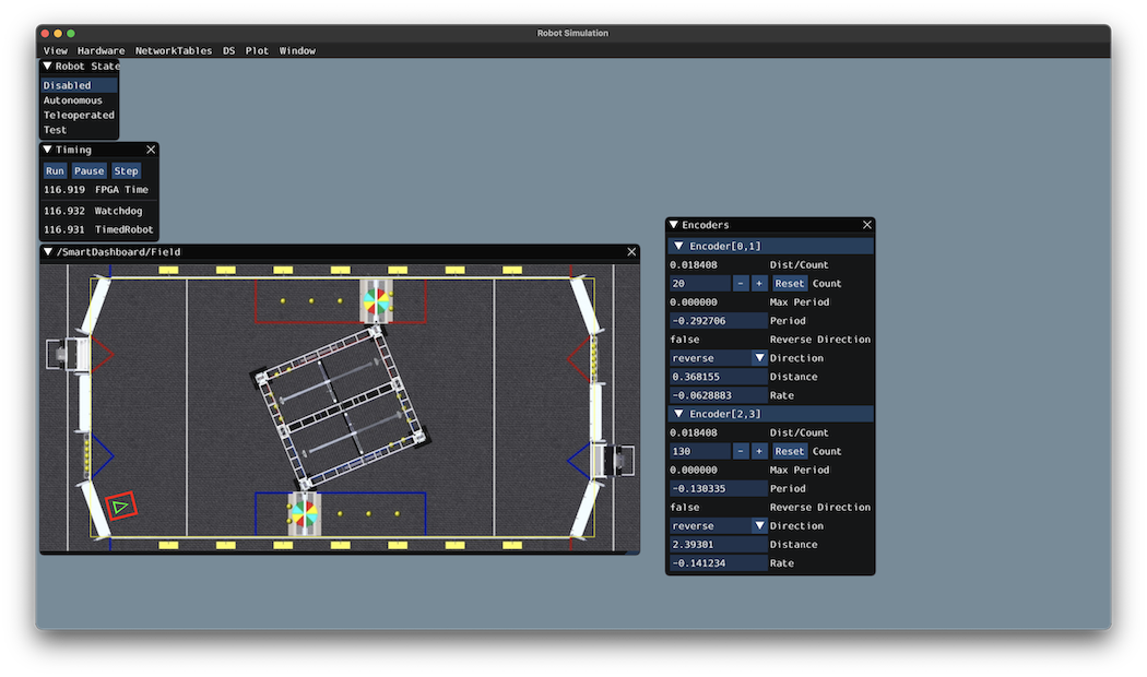
Why Simulate a Drivetrain?
The drivetrain of a robot is one of the most important mechanisms on the robot – therefore, it is important to ensure that the software powering your drivetrain is as robust as possible. By being able to simulate how a physical drivetrain responds, you can get a head start on writing quality software before you have access to the physical hardware. With the simulation framework, you can verify not only basic functionality, like making sure that the inversions on motors and encoders are correct, but also advanced capabilities such as verifying accuracy of path following.
Step 1: Creating Simulated Instances of Hardware
The WPILib simulation framework contains several XXXSim classes, where XXX represents physical hardware such as encoders or gyroscopes. These simulation classes can be used to set positions and velocities (for encoders) and angles (for gyroscopes) from a model of your drivetrain. See the Device Simulation article for more info about these simulation hardware classes and simulation of vendor devices.
Simulating Encoders
The EncoderSim class allows users to set encoder positions and velocities on a given Encoder object. When running on real hardware, the Encoder class interacts with real sensors to count revolutions (and convert them to distance units automatically if configured to do so); however, in simulation there are no such measurements to make. The EncoderSim class can accept these simulated readings from a model of your drivetrain.
Note
It is not possible to simulate encoders that are directly connected to CAN motor controllers using WPILib classes. For more information about your specific motor controller, please read your vendor’s documentation.
// These represent our regular encoder objects, which we would
// create to use on a real robot.
private Encoder m_leftEncoder = new Encoder(0, 1);
private Encoder m_rightEncoder = new Encoder(2, 3);
// These are our EncoderSim objects, which we will only use in
// simulation. However, you do not need to comment out these
// declarations when you are deploying code to the roboRIO.
private EncoderSim m_leftEncoderSim = new EncoderSim(m_leftEncoder);
private EncoderSim m_rightEncoderSim = new EncoderSim(m_rightEncoder);
#include <frc/Encoder.h>
#include <frc/simulation/EncoderSim.h>
...
// These represent our regular encoder objects, which we would
// create to use on a real robot.
frc::Encoder m_leftEncoder{0, 1};
frc::Encoder m_rightEncoder{2, 3};
// These are our EncoderSim objects, which we will only use in
// simulation. However, you do not need to comment out these
// declarations when you are deploying code to the roboRIO.
frc::sim::EncoderSim m_leftEncoderSim{m_leftEncoder};
frc::sim::EncoderSim m_rightEncoderSim{m_rightEncoder};
Simulating Gyroscopes
Similar to the EncoderSim class, simulated gyroscope classes also exist for commonly used WPILib gyros – AnalogGyroSim and ADXRS450_GyroSim. These are also constructed in the same manner.
Note
It is not possible to simulate certain vendor gyros (i.e. Pigeon IMU and NavX) using WPILib classes. Please read the respective vendors’ documentation for information on their simulation support.
// Create our gyro object like we would on a real robot.
private AnalogGyro m_gyro = new AnalogGyro(1);
// Create the simulated gyro object, used for setting the gyro
// angle. Like EncoderSim, this does not need to be commented out
// when deploying code to the roboRIO.
private AnalogGyroSim m_gyroSim = new AnalogGyroSim(m_gyro);
#include <frc/AnalogGyro.h>
#include <frc/simulation/AnalogGyroSim.h>
...
// Create our gyro objectl ike we would on a real robot.
frc::AnalogGyro m_gyro{1};
// Create the simulated gyro object, used for setting the gyro
// angle. Like EncoderSim, this does not need to be commented out
// when deploying code to the roboRIO.
frc::sim::AnalogGyroSim m_gyroSim{m_gyro};
Step 2: Creating a Drivetrain Model
In order to accurately determine how your physical drivetrain will respond to given motor voltage inputs, an accurate model of your drivetrain must be created. This model is usually created by measuring various physical parameters of your real robot. In WPILib, this drivetrain simulation model is represented by the DifferentialDrivetrainSim class.
Creating a DifferentialDrivetrainSim from Physical Measurements
One way to creating a DifferentialDrivetrainSim instance is by using physical measurements of the drivetrain and robot – either obtained through CAD software or real-world measurements (the latter will usually yield better results as it will more closely match reality). This constructor takes the following parameters:
The type and number of motors on one side of the drivetrain.
The gear ratio between the motors and the wheels as output torque over input torque (this number is usually greater than 1 for drivetrains).
The moment of inertia of the drivetrain (this can be obtained from a CAD model of your drivetrain. Usually, this is between 3 and 8 \(kg m^2\)).
The mass of the drivetrain (it is recommended to use the mass of the entire robot itself, as it will more accurately model the acceleration characteristics of your robot for trajectory tracking).
The radius of the drive wheels.
The track width (distance between left and right wheels).
Standard deviations of measurement noise: this represents how much measurement noise you expect from your real sensors. The measurement noise is an array with 7 elements, with each element representing the standard deviation of measurement noise in x, y, heading, left velocity, right velocity, left position, and right position respectively. This option can be omitted in C++ or set to
nullin Java if measurement noise is not desirable.
You can calculate the measurement noise of your sensors by taking multiple data points of the state you are trying to measure and calculating the standard deviation using a tool like Python. For example, to calculate the standard deviation in your encoders’ velocity estimate, you can move your robot at a constant velocity, take multiple measurements, and calculate their standard deviation from the known mean. If this process is too tedious, the values used in the example below should be a good representation of average noise from encoders.
Note
The standard deviation of the noise for a measurement has the same units as that measurement. For example, the standard deviation of the velocity noise has units of m/s.
Note
It is very important to use SI units (i.e. meters and radians) when passing parameters in Java. In C++, the units library can be used to specify any unit type.
// Create the simulation model of our drivetrain.
DifferentialDrivetrainSim m_driveSim = new DifferentialDrivetrainSim(
DCMotor.getNEO(2), // 2 NEO motors on each side of the drivetrain.
7.29, // 7.29:1 gearing reduction.
7.5, // MOI of 7.5 kg m^2 (from CAD model).
60.0, // The mass of the robot is 60 kg.
Units.inchesToMeters(3), // The robot uses 3" radius wheels.
0.7112, // The track width is 0.7112 meters.
// The standard deviations for measurement noise:
// x and y: 0.001 m
// heading: 0.001 rad
// l and r velocity: 0.1 m/s
// l and r position: 0.005 m
VecBuilder.fill(0.001, 0.001, 0.001, 0.1, 0.1, 0.005, 0.005));
#include <frc/simulation/DifferentialDrivetrainSim.h>
...
// Create the simulation model of our drivetrain.
frc::sim::DifferentialDrivetrainSim m_driveSim{
frc::DCMotor::GetNEO(2), // 2 NEO motors on each side of the drivetrain.
7.29, // 7.29:1 gearing reduction.
7.5_kg_sq_m, // MOI of 7.5 kg m^2 (from CAD model).
60_kg, // The mass of the robot is 60 kg.
3_in, // The robot uses 3" radius wheels.
0.7112_m, // The track width is 0.7112 meters.
// The standard deviations for measurement noise:
// x and y: 0.001 m
// heading: 0.001 rad
// l and r velocity: 0.1 m/s
// l and r position: 0.005 m
{0.001, 0.001, 0.001, 0.1, 0.1, 0.005, 0.005}};
Creating a DifferentialDrivetrainSim from Characterization Gains
You can also use the gains produced by robot characterization, which you may have performed as part of setting up the trajectory tracking workflow outlined here to create a simulation model of your drivetrain and often yield results closer to real-world behavior than the method above.
Important
You must need two sets of Kv and Ka gains from the characterization tool – one from straight-line motion and the other from rotating in place. We will refer to these two sets of gains as linear and angular gains respectively.
This constructor takes the following parameters:
A linear system representing the drivetrain – this can be created using the characterization gains.
The track width (distance between the left and right wheels).
The type and number of motors on one side of the drivetrain.
The gear ratio between the motors and the wheels as output torque over input torque (this number is usually greater than 1 for drivetrains).
The radius of the drive wheels.
Standard deviations of measurement noise: this represents how much measurement noise you expect from your real sensors. The measurement noise is an array with 7 elements, with each element representing the standard deviation of measurement noise in x, y, heading, left velocity, right velocity, left position, and right position respectively. This option can be omitted in C++ or set to
nullin Java if measurement noise is not desirable.
You can calculate the measurement noise of your sensors by taking multiple data points of the state you are trying to measure and calculating the standard deviation using a tool like Python. For example, to calculate the standard deviation in your encoders’ velocity estimate, you can move your robot at a constant velocity, take multiple measurements, and calculate their standard deviation from the known mean. If this process is too tedious, the values used in the example below should be a good representation of average noise from encoders.
Note
The standard deviation of the noise for a measurement has the same units as that measurement. For example, the standard deviation of the velocity noise has units of m/s.
Note
It is very important to use SI units (i.e. meters and radians) when passing parameters in Java. In C++, the units library can be used to specify any unit type.
// Create our feedforward gain constants (from the characterization
// tool)
static final double KvLinear = 1.98;
static final double KaLinear = 0.2;
static final double KvAngular = 1.5;
static final double KaAngular = 0.3;
// Create the simulation model of our drivetrain.
private DifferentialDrivetrainSim m_driveSim = new DifferentialDrivetrainSim(
// Create a linear system from our characterization gains.
LinearSystemId.identifyDrivetrainSystem(KvLinear, KaLinear, KvAngular, KaAngular),
DCMotor.getNEO(2), // 2 NEO motors on each side of the drivetrain.
7.29, // 7.29:1 gearing reduction.
0.7112, // The track width is 0.7112 meters.
Units.inchesToMeters(3), // The robot uses 3" radius wheels.
// The standard deviations for measurement noise:
// x and y: 0.001 m
// heading: 0.001 rad
// l and r velocity: 0.1 m/s
// l and r position: 0.005 m
VecBuilder.fill(0.001, 0.001, 0.001, 0.1, 0.1, 0.005, 0.005));
#include <frc/simulation/DifferentialDrivetrainSim.h>
#include <frc/system/plant/LinearSystemId.h>
#include <units/acceleration.h>
#include <units/angular_acceleration.h>
#include <units/angular_velocity.h>
#include <units/voltage.h>
#include <units/velocity.h>
...
// Create our feedforward gain constants (from the characterization
// tool). Note that these need to have correct units.
static constexpr auto KvLinear = 1.98_V / 1_mps;
static constexpr auto KaLinear = 0.2_V / 1_mps_sq;
static constexpr auto KvAngular = 1.5_V / 1_rad_per_s;
static constexpr auto KaAngular = 0.3_V / 1_rad_per_s_sq;
// Create the simulation model of our drivetrain.
frc::sim::DifferentialDrivetrainSim m_driveSim{
// Create a linear system from our characterization gains.
frc::LinearSystemId::IdentifyDrivetrainSystem(
KvLinear, KaLinear, KvAngular, KaAngular),
0.7112_m, // The track width is 0.7112 meters.
frc::DCMotor::GetNEO(2), // 2 NEO motors on each side of the drivetrain.
7.29, // 7.29:1 gearing reduction.
3_in, // The robot uses 3" radius wheels.
// The standard deviations for measurement noise:
// x and y: 0.001 m
// heading: 0.001 rad
// l and r velocity: 0.1 m/s
// l and r position: 0.005 m
{0.001, 0.001, 0.001, 0.1, 0.1, 0.005, 0.005}};
Creating a DifferentialDrivetrainSim of the KoP Chassis
The DifferentialDrivetrainSim class also has a static createKitbotSim() (Java) / CreateKitbotSim() (C++) method that can create an instance of the DifferentialDrivetrainSim using the standard Kit of Parts Chassis parameters. This method takes 5 arguments, two of which are optional:
The type and number of motors on one side of the drivetrain.
The gear ratio between the motors and the wheels as output torque over input torque (this number is usually greater than 1 for drivetrains).
The diameter of the wheels installed on the drivetrain.
The moment of inertia of the drive base (optional).
Standard deviations of measurement noise: this represents how much measurement noise you expect from your real sensors. The measurement noise is an array with 7 elements, with each element representing the standard deviation of measurement noise in x, y, heading, left velocity, right velocity, left position, and right position respectively. This option can be omitted in C++ or set to
nullin Java if measurement noise is not desirable.
You can calculate the measurement noise of your sensors by taking multiple data points of the state you are trying to measure and calculating the standard deviation using a tool like Python. For example, to calculate the standard deviation in your encoders’ velocity estimate, you can move your robot at a constant velocity, take multiple measurements, and calculate their standard deviation from the known mean. If this process is too tedious, the values used in the example below should be a good representation of average noise from encoders.
Note
The standard deviation of the noise for a measurement has the same units as that measurement. For example, the standard deviation of the velocity noise has units of m/s.
Note
It is very important to use SI units (i.e. meters and radians) when passing parameters in Java. In C++, the units library can be used to specify any unit type.
private DifferentialDrivetrainSim m_driveSim = DifferentialDrivetrainSim.createKitbotSim(
KitbotMotor.kDualCIMPerSide, // 2 CIMs per side.
KitbotGearing.k10p71, // 10.71:1
KitbotWheelSize.SixInch, // 6" diameter wheels.
null // No measurement noise.
);
#include <frc/simulation/DifferentialDrivetrainSim.h>
...
frc::sim::DifferentialDrivetrainSim m_driveSim =
frc::sim::DifferentialDrivetrainSim::CreateKitbotSim(
frc::sim::DifferentialDrivetrainSim::KitbotMotor::DualCIMPerSide, // 2 CIMs per side.
frc::sim::DifferentialDrivetrainSim::KitbotGearing::k10p71, // 10.71:1
frc::sim::DifferentialDrivetrainSim::KitbotWheelSize::kSixInch // 6" diameter wheels.
);
Note
You can use the KitbotMotor, KitbotGearing, and KitbotWheelSize enum (Java) / struct (C++) to get commonly used configurations of the Kit of Parts Chassis.
Important
Constructing your DifferentialDrivetrainSim instance in this way is just an approximation and is intended to get teams quickly up and running with simulation. Using empirical values measured from your physical robot will always yield more accurate results.
Step 3: Updating the Drivetrain Model
Now that the drivetrain model has been made, it needs to be updated periodically with the latest motor voltage commands. It is recommended to do this step in a separate simulationPeriodic() / SimulationPeriodic() method inside your subsystem and only call this method in simulation.
Note
If you are using the command-based framework, every subsystem that extends SubsystemBase has a simulationPeriodic() / SimulationPeriodic() which can be overridden. This method is automatically run only during simulation. If you are not using the command-based library, make sure you call your simulation method inside the overridden simulationPeriodic() / SimulationPeriodic() of the main Robot class. These periodic methods are also automatically called only during simulation.
There are three main steps to updating the model:
Set the input of the drivetrain model. These are the motor voltages from the two sides of the drivetrain.
Advance the model forward in time by the nominal periodic timestep (Usually 20 ms). This updates all of the drivetrain’s states (i.e. pose, encoder positions and velocities) as if 20 ms had passed.
Update simulated sensors with new positions, velocities, and angles to use in other places.
private PWMSparkMax m_leftMotor = new PWMSparkMax(0);
private PWMSparkMax m_rightMotor = new PWMSparkMax(1);
public Drivetrain() {
...
m_leftEncoder.setDistancePerPulse(2 * Math.PI * kWheelRadius / kEncoderResolution);
m_rightEncoder.setDistancePerPulse(2 * Math.PI * kWheelRadius / kEncoderResolution);
}
public void simulationPeriodic() {
// Set the inputs to the system. Note that we need to convert
// the [-1, 1] PWM signal to voltage by multiplying it by the
// robot controller voltage.
m_driveSim.setInputs(m_leftMotor.get() * RobotController.getInputVoltage(),
m_rightMotor.get() * RobotController.getInputVoltage());
// Advance the model by 20 ms. Note that if you are running this
// subsystem in a separate thread or have changed the nominal timestep
// of TimedRobot, this value needs to match it.
m_driveSim.update(0.02);
// Update all of our sensors.
m_leftEncoderSim.setDistance(m_driveSim.getLeftPositionMeters());
m_leftEncoderSim.setRate(m_driveSim.getLeftVelocityMetersPerSecond());
m_rightEncoderSim.setDistance(m_driveSim.getRightPositionMeters());
m_rightEncoderSim.setRate(m_driveSim.getRightVelocityMetersPerSecond());
m_gyroSim.setAngle(-m_driveSim.getHeading().getDegrees());
}
frc::PWMSparkMax m_leftMotor{0};
frc::PWMSparkMax m_rightMotor{1};
Drivetrain() {
...
m_leftEncoder.SetDistancePerPulse(2 * wpi::math::pi * kWheelRadius / kEncoderResolution);
m_rightEncoder.SetDistancePerPulse(2 * wpi::math::pi * kWheelRadius / kEncoderResolution);
}
void SimulationPeriodic() {
// Set the inputs to the system. Note that we need to convert
// the [-1, 1] PWM signal to voltage by multiplying it by the
// robot controller voltage.
m_driveSim.SetInputs(
m_leftMotor.get() * units::volt_t(frc::RobotController::GetInputVoltage()),
m_rightMotor.get() * units::volt_t(frc::RobotController::GetInputVoltage()));
// Advance the model by 20 ms. Note that if you are running this
// subsystem in a separate thread or have changed the nominal timestep
// of TimedRobot, this value needs to match it.
m_driveSim.Update(20_ms);
// Update all of our sensors.
m_leftEncoderSim.SetDistance(m_driveSim.GetLeftPosition().value());
m_leftEncoderSim.SetRate(m_driveSim.GetLeftVelocity().value());
m_rightEncoderSim.SetDistance(m_driveSim.GetRightPosition().value());
m_rightEncoderSim.SetRate(m_driveSim.GetRightVelocity().value());
m_gyroSim.SetAngle(-m_driveSim.GetHeading().Degrees());
}
Important
If the right side of your drivetrain is inverted, you MUST negate the right voltage in the SetInputs() call to ensure that positive voltages correspond to forward movement.
Important
Because the drivetrain simulator model returns positions and velocities in meters and m/s respectively, these must be converted to encoder ticks and ticks/s when calling SetDistance() and SetRate(). Alternatively, you can configure SetDistancePerPulse on the encoders to have the Encoder object take care of this automatically – this is the approach that is taken in the example above.
Now that the simulated encoder positions, velocities, and gyroscope angles have been set, you can call m_leftEncoder.GetDistance(), etc. in your robot code as normal and it will behave exactly like it would on a real robot. This involves performing odometry calculations, running velocity PID feedback loops for trajectory tracking, etc.
Step 4: Updating Odometry and Visualizing Robot Position
Now that the simulated encoder positions, velocities, and gyro angles are being updated with accurate information periodically, this data can be used to update the pose of the robot in a periodic loop (such as the periodic() method in a Subsystem). In simulation, the periodic loop will use simulated encoder and gyro readings to update odometry whereas on the real robot, the same code will use real readings from physical hardware.
Note
For more information on using odometry, see this document.
Robot Pose Visualization
The robot pose can be visualized on the Simulator GUI (during simulation) or on a dashboard such as Glass (on a real robot) by sending the odometry pose over a Field2d object. A Field2d can be trivially constructed without any constructor arguments:
private Field2d m_field = new Field2d();
#include <frc/smartdashboard/Field2d.h>
..
frc::Field2d m_field;
This Field2d instance must then be sent over NetworkTables. The best place to do this is in the constructor of your subsystem.
public Drivetrain() {
...
SmartDashboard.putData("Field", m_field);
}
#include <frc/smartdashboard/SmartDashboard.h>
Drivetrain() {
...
frc::SmartDashboard::PutData("Field", &m_field);
}
Note
The Field2d instance can also be sent using a lower-level NetworkTables API or using the Shuffleboard API.
Finally, the pose from your odometry must be updated periodically into the Field2d object. Remember that this should be in a general periodic() method i.e. one that runs both during simulation and during real robot operation.
public void periodic() {
...
// This will get the simulated sensor readings that we set
// in the previous article while in simulation, but will use
// real values on the robot itself.
m_odometry.update(m_gyro.getRotation2d(),
m_leftEncoder.getDistance(),
m_rightEncoder.getDistance());
m_field.setRobotPose(m_odometry.getPoseMeters());
}
void Periodic() {
...
// This will get the simulated sensor readings that we set
// in the previous article while in simulation, but will use
// real values on the robot itself.
m_odometry.Update(m_gyro.GetRotation2d(),
units::meter_t(m_leftEncoder.GetDistance()),
units::meter_t(m_rightEncoder.GetDistance()));
m_field.SetRobotPose(m_odometry.GetPose());
}
Important
It is important that this code is placed in a regular periodic() method – one that is called periodically regardless of mode of operation. If you are using the command-based library, this method already exists. If not, you are responsible for calling this method periodically from the main Robot class.
Note
At this point we have covered all of the code changes required to run your code. You should head to the Simulation User Interface page for more info on how to run the simulation and add the field that your simulated robot will run on to the GUI.
Unit Testing
Unit testing is a method of testing code by dividing the code into the smallest “units” possible and testing each unit. In robot code, this can mean testing the code for each subsystem individually. There are many unit testing frameworks for most languages. Java robot projects have JUnit 4 available by default, and C++ robot projects have Google Test.
Writing Testable Code
Note
This example can be easily adapted to the command-based paradigm by having Intake inherit from SubsystemBase.
Our subsystem will be an Infinite Recharge intake mechanism containing a piston and a motor: the piston deploys/retracts the intake, and the motor will pull the Power Cells inside. We don’t want the motor to run if the intake mechanism isn’t deployed because it won’t do anything.
To provide a “clean slate” for each test, we need to have a function to destroy the object and free all hardware allocations. In Java, this is done by implementing the AutoCloseable interface and its .close() method, destroying each member object by calling the member’s .close() method - an object without a .close() method probably doesn’t need to be closed. In C++, the default destructor will be called automatically when the object goes out of scope and will call destructors of member objects.
Note
Vendors might not support resource closing identically to the way shown here. See your vendor’s documentation for more information as to what they support and how.
import edu.wpi.first.wpilibj.DoubleSolenoid;
import edu.wpi.first.wpilibj.PWMSparkMax;
import frc.robot.Constants.IntakeConstants;
public class Intake implements AutoCloseable {
private PWMSparkMax motor;
private DoubleSolenoid piston;
public Intake() {
motor = new PWMSparkMax(IntakeConstants.MOTOR_PORT);
piston = new DoubleSolenoid(PneumaticsModuleType.CTREPCM, IntakeConstants.PISTON_FWD, IntakeConstants.PISTON_REV);
}
public void deploy() {
piston.set(DoubleSolenoid.Value.kForward);
}
public void retract() {
piston.set(DoubleSolenoid.Value.kReverse);
motor.set(0); // turn off the motor
}
public void activate(double speed) {
if (piston.get() == DoubleSolenoid.Value.kForward) {
motor.set(speed);
} else { // if piston isn't open, do nothing
motor.set(0);
}
}
@Override
public void close() throws Exception {
piston.close();
motor.close();
}
}
#include <frc2/command/SubsystemBase.h>
#include <frc/DoubleSolenoid.h>
#include <frc/PWMSparkMax.h>
#include "Constants.h"
class Intake : public frc2::SubsystemBase {
public:
void Deploy();
void Retract();
void Activate(double speed);
private:
frc::PWMSparkMax motor{Constants::Intake::MOTOR_PORT};
frc::DoubleSolenoid piston{frc::PneumaticsModuleType::CTREPCM, Constants::Intake::PISTON_FWD, Constants::Intake::PISTON_REV};
};
#include "subsystems/Intake.h"
void Intake::Deploy() {
piston.Set(frc::DoubleSolenoid::Value::kForward);
}
void Intake::Retract() {
piston.Set(frc::DoubleSolenoid::Value::kReverse);
motor.Set(0); // turn off the motor
}
void Intake::Activate(double speed) {
if (piston.Get() == frc::DoubleSolenoid::Value::kForward) {
motor.Set(speed);
} else { // if piston isn't open, do nothing
motor.Set(0);
}
}
Writing Tests
Important
Tests are placed inside the test source set: /src/test/java/ and /src/test/cpp/ for Java and C++ tests, respectively. Files outside that source root do not have access to the test framework - this will fail compilation due to unresolved references.
In Java, each test class contains at least one test method marked with @org.junit.Test, each method representing a test case. Additional methods for opening resources (such as our Intake object) before each test and closing them after are respectively marked with @org.junit.Before and @org.junit.After. In C++, test fixture classes inheriting from testing::Test contain our subsystem and simulation hardware objects, and test methods are written using the TEST_F(testfixture, testname) macro. The SetUp() and TearDown() methods can be overridden in the test fixture class and will be run respectively before and after each test.
Each test method should contain at least one assertion (assert*() in Java or EXPECT_*() in C++). These assertions verify a condition at runtime and fail the test if the condition isn’t met. If there is more than one assertion in a test method, the first failed assertion will crash the test - execution won’t reach the later assertions.
Both JUnit and GoogleTest have multiple assertion types, but the most common is equality: assertEquals(expected, actual)/EXPECT_EQ(expected, actual). When comparing numbers, a third parameter - delta, the acceptable error, can be given. In JUnit (Java), these assertions are static methods and can be used without qualification by adding the static star import import static org.junit.Asssert.*. In Google Test (C++), assertions are macros from the <gtest/gtest.h> header.
Note
Comparison of floating-point values isn’t accurate, so comparing them should be done with an acceptable error parameter (DELTA).
import static org.junit.Assert.*;
import edu.wpi.first.hal.HAL;
import edu.wpi.first.wpilibj.DoubleSolenoid;
import edu.wpi.first.wpilibj.simulation.DoubleSolenoidSim;
import edu.wpi.first.wpilibj.simulation.PWMSim;
import frc.robot.Constants.IntakeConstants;
import org.junit.*;
public class IntakeTest {
public static final double DELTA = 1e-2; // acceptable deviation range
Intake intake;
PWMSim simMotor;
DoubleSolenoidSim simPiston;
@Before // this method will run before each test
public void setup() {
assert HAL.initialize(500, 0); // initialize the HAL, crash if failed
intake = new Intake(); // create our intake
simMotor = new PWMSim(IntakeConstants.MOTOR_PORT); // create our simulation PWM motor controller
simPiston = new DoubleSolenoidSim(PneumaticsModuleType.CTREPCM, IntakeConstants.PISTON_FWD, IntakeConstants.PISTON_REV); // create our simulation solenoid
}
@After // this method will run after each test
public void shutdown() throws Exception {
intake.close(); // destroy our intake object
}
@Test // marks this method as a test
public void doesntWorkWhenClosed() {
intake.retract(); // close the intake
intake.activate(0.5); // try to activate the motor
assertEquals(0.0, simMotor.getSpeed(), DELTA); // make sure that the value set to the motor is 0
}
@Test
public void worksWhenOpen() {
intake.deploy();
intake.activate(0.5);
assertEquals(0.5, simMotor.getSpeed(), DELTA);
}
@Test
public void retractTest() {
intake.retract();
assertEquals(DoubleSolenoid.Value.kReverse, simPiston.get());
}
@Test
public void deployTest() {
intake.deploy();
assertEquals(DoubleSolenoid.Value.kForward, simPiston.get());
}
}
#include <gtest/gtest.h>
#include <frc/DoubleSolenoid.h>
#include <frc/simulation/DoubleSolenoidSim.h>
#include <frc/simulation/PWMSim.h>
#include "subsystems/Intake.h"
#include "Constants.h"
class IntakeTest : public testing::Test {
protected:
Intake intake; // create our intake
frc::sim::PWMSim simMotor{Constants::Intake::MOTOR_PORT}; // create our simulation PWM
frc::sim::DoubleSolenoidSim simPiston{frc::PneumaticsModuleType::CTREPCM, Constants::Intake::PISTON_FWD, Constants::Intake::PISTON_REV}; // create our simulation solenoid
};
TEST_F(IntakeTest, DoesntWorkWhenClosed) {
intake.Retract(); // close the intake
intake.Activate(0.5); // try to activate the motor
EXPECT_DOUBLE_EQ(0.0, simMotor.GetSpeed()); // make sure that the value set to the motor is 0
}
TEST_F(IntakeTest, WorksWhenOpen) {
intake.Deploy();
intake.Activate(0.5);
EXPECT_DOUBLE_EQ(0.5, simMotor.GetSpeed());
}
TEST_F(IntakeTest, RetractTest) {
intake.Retract();
EXPECT_EQ(frc::DoubleSolenoid::Value::kReverse, simPiston.Get());
}
TEST_F(IntakeTest, DeployTest) {
intake.Deploy();
EXPECT_EQ(frc::DoubleSolenoid::Value::kForward, simPiston.Get());
}
For more advanced usage of JUnit and Google Test, see the framework docs.
Running Tests
Note
Tests will always be run in simulation on your desktop. For prerequisites and more info, see the simulation introduction.
For Java tests to run, make sure that your build.gradle file contains the following block:
test {
useJUnit()
}
Use Test Robot Code from the Command Palette to run the tests. Results will be reported in the terminal output, each test will have a FAILED or PASSED/OK label next to the test name in the output. JUnit (Java only) will generate a HTML document in build/reports/tests/test/index.html with a more detailed overview of the results; if there are failied test a link to render the document in your browser will be printed in the terminal output.
By default, Gradle runs the tests whenever robot code is built, including deploys. This will increase deploy time, and failing tests will cause the build and deploy to fail. To prevent this from happening, you can use Change Skip Tests On Deploy Setting from the Command Palette to configure whether to run tests when deploying.
OutlineViewer
OutlineViewer is a utility used to view, modify and add to the contents of the NetworkTables for debugging purposes. It displays all key value pairs currently in the NetworkTables and can be used to modify the value of existing keys or add new keys to the table. OutlineViewer is included in the Java and C++ language installations.
In Visual Studio Code, press Ctrl+Shift+P and type WPILib or click the WPILib logo in the top right to launch the WPILib Command Palette. Select Start Tool, then select OutlineViewer.
To connect to your robot, open OutlineViewer and set the Server Location to be your team number. After you click start, OutlineViewer will connect. If you have trouble connecting to OutlineViewer please see the Dashboard Troubleshooting Steps.
Note
You can use localhost instead of a team number to point OutlineViewer at a simulated robot or a Romi.
To add additional key/value pairs to NetworkTables, right click on a location and choose the corresponding data type.
Note
LabVIEW teams can use the Variables tab of the LabVIEW Dashboard to accomplish the same functionality as OutlineViewer.
Axon
Introduction to Axon
Axon is a tool that brings machine learning to the FIRST robotics competition. Axon provides an interface for training, testing, and exporting a machine learning model.
What is Machine Learning?
Machine learning is a new, exciting field of computer science. Machine learning is a powerful tool that can accomplish computational tasks that traditional algorithms cannot. In the FIRST Robotics Competition, machine learning can be used to detect game pieces, scoring locations, or even other robots.
A machine learning solution is better than traditional computer vision algorithms in many scenarios. The patterns that a machine learning algorithm (in this case, a neural network) can recognize can be much more complex than what an HSV-filtering algorithm can recognize. For example, a neural network could detect the location of a FRC robot within an image, which is an unreasonable challenge for a HSV-filtering algorithm.
Object detection is a field of machine learning that is particularly relevant for the FRC use-case. A neural network can be taught to determine the box that surrounds an object within an image. This box is known as a bounding box. An object detection neural network is given an image, and it provides a set of predictions. Each prediction contains a bounding box, a label of what the object is, and a number representing how confident the neural network is that there is the chosen object within that bounding box.
Features of Axon
Dataset Viewing
Machine learning requires giant datasets for the machines to recognize patterns in real-world data. The Axon tool supports custom datasets made with Supervisely. It also supports datasets made from a slice of the Open Images dataset, a Google dataset made of over 6 million images of generic objects. Please go to the dataset page to see how to upload a supported dataset format.
Training
Axon provides an excellent UI for doing transfer learning with a quantised COCO-trained MobileNet V2. Transfer learning is a technique that reuses parts of a previously trained model, a MobileNet v2 in this case, to improve the learning of a new task like locating hatch panels. Real-time metrics are provided, showing the precision of your model.
Testing
Axon provides a way to test a trained model before using it on a robot. Simply upload a video to the testing page, and watch the neural network work in real-time. A .mp4 is provided when testing is complete, if so desired.
Exporting
Axon provides a way to export your model in both a normal TFLite format, as well as a Edge-TPU optimized model. The outputted .zip can be directly uploaded to the WPILib Raspberry Pi image, but the format works on many other platforms.
Inferencing
Axon provides a Python script for running models on a coprocessor. This script will utilize the hardware of a Google Coral Edge TPU if there is one plugged in. The is officially supported on the WPILibPi image. All inference data is outputted over NetworkTables, and an output MJPEG stream is also provided.
Installation
Docker
Docker is a system that allows for virtual machines to be run in containers. Machine Learning utilizes many difficult to install dependencies, so we have provided docker containers to make this installation painless.
To install docker visit the link and installation instructions provided here: Docker Desktop
For Windows users an installation of Windows Subsystem for Linux (WSL) is required and can be found here
For Mac users, follow these instructions to increase Memory allowance to at least 6GBs of RAM. Instructions can be found here
For Linux users, follow these instructions to complete the installation.
Introduction to Machine Learning
Machine learning is a giant optimization problem. A neural network is a series of matrices, where the number contained within the matrices need to be tuned as precisely as possible to make the best predictions possible. To understand what this means better, let’s look at a classic machine learning problem: MNIST.
MNIST
MNIST (“Modified National Institute of Standards and Technology”) is a commonly used datatset in Computer Vision that deals with classification. The dataset itself is a collection of images showing hand-drawn numbers. The challenge is to create an algorithm that can recognize what number is represented by a given image, which is solvable by developing a neural network.
Here we have an over-simplified neural network. It has three layers, arranged vertically. The furthest left layer is called the input layer. When feeding an image into the neural network, the input layer is set to have the same values as our image. The middle layer is called a hidden layer. This layer focuses on computation, and does not directly interact with by the programmer. The final layer in this neural network is called the output layer and contains the end result.
Having discussed the nodes (the circles) that make up the layers, it is important to discuss the connections (the arrows) between the layers. Each arrow represents a set of operations between two nodes. This type of neural network is a fully-connected neural network, so the operations that the arrows represent are shown below.
Where \(Y\) is a non-input matrix layer, and \(X\) is the matrix directly before (to the left) of \(Y\). \(W\) is a matrix of weights that act as coefficients on \(X\). \(b\) is a matrix of biases that add to the result of the product of \(W\) and \(X\). During the training/learning process, the values within \(W\) and \(b\) are adjusted so \(Y\) is the best possible value from any \(X\). In a large neural network, there are millions of weights and biases, resulting in billions of linear algebra operations. This absurd amount math often requires a powerful computer, and/or a lot of time.
With this understanding of a basic neural network, let’s look at a simple neural network that can be used for the MNIST problem.
This neural network has an input layer, one hidden layer, and an output layer. The input layer is made of 784 nodes, as the MNIST dataset is made out of pictures that are 28x28 pixels. Each pixel is either 0 or 1. This input layer is multiplied by a weights matrix and a bias matrix is added, resulting in the hidden layer. The hidden layer is multiplied by another weight matrix and another bias matrix is added, resulting in the output layer. The output layer is made of exactly 10 nodes, representing 0 through 9. The actual value of each node represents the confidence of that node being correct. For example, if node 0 has a value of .91, and node 1 has a value of .23, then the input image is more likely a 0 than a 1.
MobileNet V2
The neural network that Axon uses is much more complex than the one described for the MNIST problem. It is a convolutional neural network (CNN), distinctly different than the fully-connected neural network used for MNIST.
If you would like to learn more about the MobileNet architecture, you can read here. This knowledge is not necessary to use Axon to successfully deploy a neural network on your robot.
Labeling a Dataset with Supervisely
The quality of a neural network is fully dependent on the quality of the dataset used to train it. To create a custom dataset, perhaps to train a neural network to recognize the new game piece, Axon supports datasets created using Supervisely. This page describes how to create label, and export a dataset made with Supervisely.
Record a Video
The first step to creating a dataset is getting images. A dataset should have several thousand images. To get this many images, the easiest way is to record a short video, roughly 1 to 5 minutes long. The video should clearly display the object(s) you wish to detect in several angles. Below is an example clip of a video used to teach a neural network to recognize a video game controller.
Import Video to Supervisely
Now that the images for the dataset are gathered, they can be labeled. To do this, Axon supports the use of https://supervise.ly . An account is required to use the site.
The workflow is organized in Workspaces, and Projects. A Workspace can have multiple users, so one FRC team can share a workspace. A Workspace also can contain multiple projects.
Inside of a Workspace, the video recorded in the previous step can be imported.
In the import page, the most important step is choosing the correct Import plugin. The correct plugin is “Videos (split into frames).” The setting configurations do not need to be changed.
With the correct plugin selected, the video can be dragged in to the upload box. This will upload the video to Supervisely, and move to a different screen (shown below). Here, the project should be given a name, and the import should be started, which will convert the video into several thousand individual images.
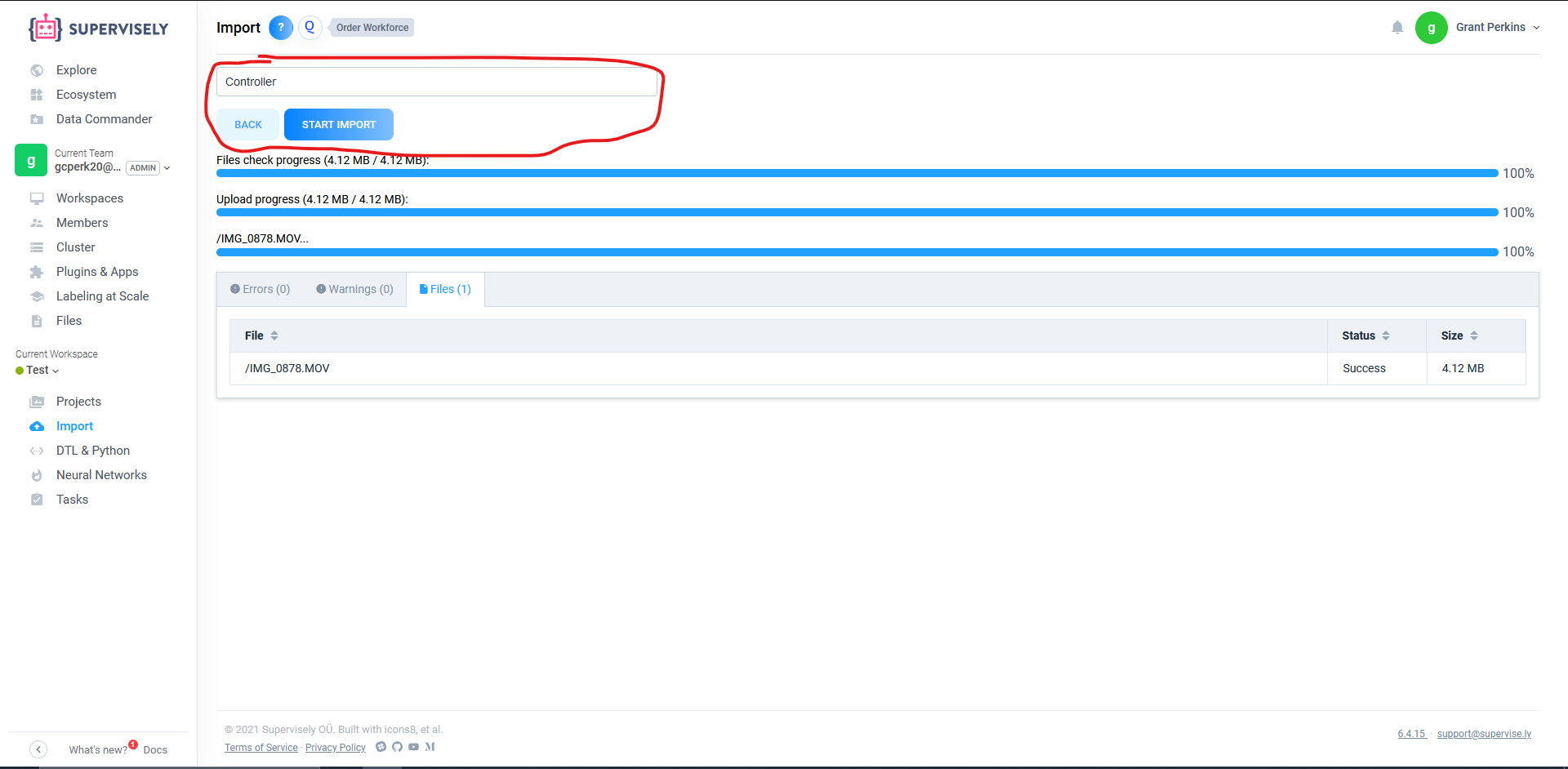
Labeling the Images
With the project now set up, the data can be labeled. Labeling data means drawing boxes around the objects a neural network would want to detect, so the neural network knows when it is right and when it is wrong when it tries to detect where an object is. The boxes drawn should tightly wrap the entire visible object within each image.
Within the Project, select the Rectangle tool. Supervisely will prompt you to create a class, i.e. define what kind of object you are about to label. More classes can be made later. Then, click twice in opposite corners around the object you wish to label. An example of a good label is below.
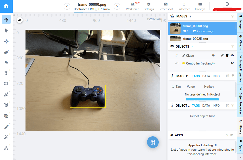
Click the Rectangle tool to label another object within the same image, if there is one. If there is a misclick, the corners of the rectangle can be dragged to better label the object. Otherwise, move on to the next image. It is important to label every single visible object that one wishes to detect, else the neural network will pick up bad habits. The job of labeling data can be tedious, but it can also be shared between members of an FRC team through the Workspace.
Downloading the Dataset
With all the images labeled, the dataset can be downloaded off of Supervisely for use in Axon. Within the Workspace, click on the triple-dot icon of the project you wish to download. Select the .json and images download option.
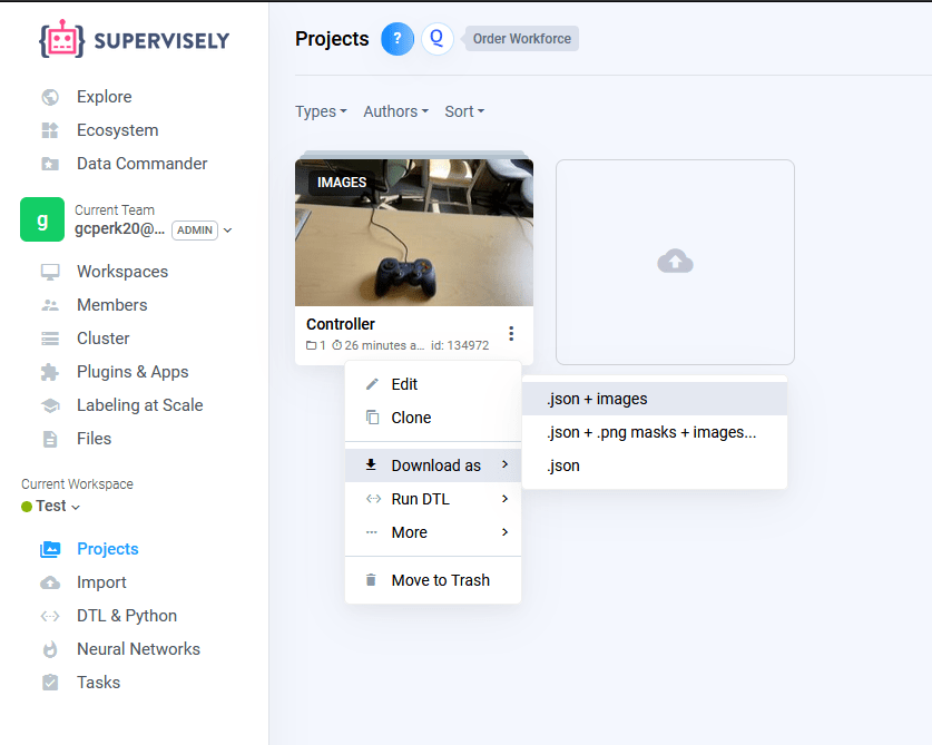
You are now ready to begin training a neural network.
Creating a Dataset with Open Images
For the detection of more generic objects, Axon’s dataset creator can be used to make a dataset from Google’s Open Images dataset .
Creating a Dataset
Click the Create Dataset button to begin.
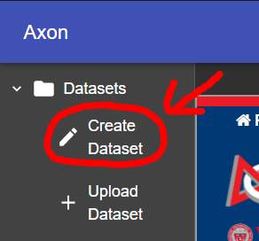
Choosing the Class Names
Next, you need to pick the classes that you would like to detect. They must be selected from the classes available at the Open Images dataset website . Change the category in the top bar to see available classes. In the below picture, Cat is selected, but other class names like Caterpillar are shown to be valid.
When you have determined the valid class names of the objects that you wish to detect, you can type them into dialog as shown below.
Furthermore, using the add button, you can choose to make a dataset containing more than one class. Subsequently, you can also remove classes using the remove button.
Choosing the Number of Images
Finally, you can select the amount of images that you want for each class category in your dataset and click CREATE.
Waiting
The creation process will take from a couple seconds to several minutes, depending on the size of your dataset. The newly-created dataset will be automatically imported into the dataset pane on the left side of the screen, but there is a Download button for sending the dataset to a teammate.
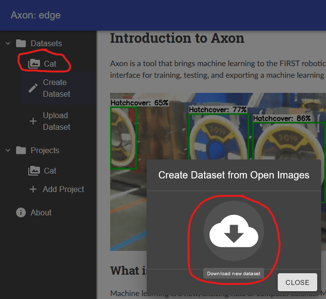
Viewing Datasets in Axon
Axon allows for the viewing of supervisely and open-images datasets.
Stats
Clicking on a dataset in the pane on the left will allow you to view all the images in the dataset. The size of the set and the classnames/labels in the dataset are displayed.
Navigation
All the images will be displayed 48 to a page. You can use the pagination navigator at the bottom to move through large datasets and find specific images if desired.

Retraining Mobilenet V2
Upload a Dataset
To retrain the mobilenet object detection model using Axon, first upload the dataset you would like to retrain with.
Once you have uploaded a dataset, you should see it in the tree above this button.
Create a Project
Next, you must create a project. A project will hold the data from the retraining, and any TFLite exports or tests you create with the retrained model.
To create a project, click the Add Project button.
A dialog will appear, asking you to name the project. Pick a name and click Create. When you create your project, you will see it above the button to the left.
Click on the project, and you will be taken to its page.
Start Retraining
At the top of the project window, there are several parameters to specify how you want the model to be retrained.
Epochs: The number of times the dataset will be passed through the model during training. Generally more epochs are better, and a model should continue to be trained until the performance increase becomes very small or it stops improving.
Batch Size: The amount of images to use in each training iteration. A larger batch size will make epochs train faster as there will be less batches, but it will require more memory to load all of the images. Generally we recommend leaving this value at default.
Evaluation Frequency: The amount of epochs to run before each evaluation of the models precision. Each evaluation will be viewable so you can check the progress of your model.
Percent Evaluation: The percent of the dataset to be reserved exclusively for evaluation of the models precision during training. A higher percent evaluation means that more images are used to test the model. Those images will not be used to train the model so there will be less training data. Generally we recommend leaving this value at default.
Datasets: The datasets you would wish to retrain with. Edit these input parameters to fit your needs, and tick the checkboxes of the desired datasets from the dropdown.
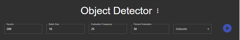
When you are ready to start the retraining, click the play button to the right of the dataset dropdown.
When an evaluation happens, a checkpoint is produced. This is a copy of the model at a particular point in the training. While the model trains, you will see checkpoints appear as points on the graph.
Exporting a Checkpoint in TFLite Format
To export a checkpoint as a TFLite model for use, select the desired checkpoint by clicking the point on the graph.
This will select the checkpoint. Export this checkpoint by clicking the export button below the graph.
You will soon see an export appear below the button.

When the export has completed, you will see the checkpoint appear in the checkpoint menu where you can select and work with any of the exported checkpoints.
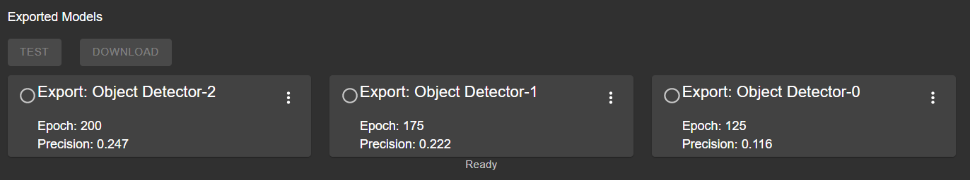
You may click the menu to the right of an exported model, providing options to rename, and delete.
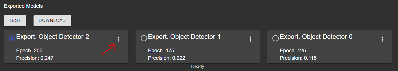
Click the download button, and your browser will download a tarfile containing two TFLite models of the selected checkpoint, one of which is optimized for the Coral TPU. There is also a label map file, for use when converting the model’s output to a human-readable format.
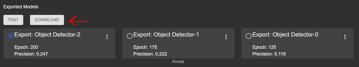
Testing an Exported Model
To test an exported model, open the testing dialog by clicking the Test button in the menu of the export you would like to test.
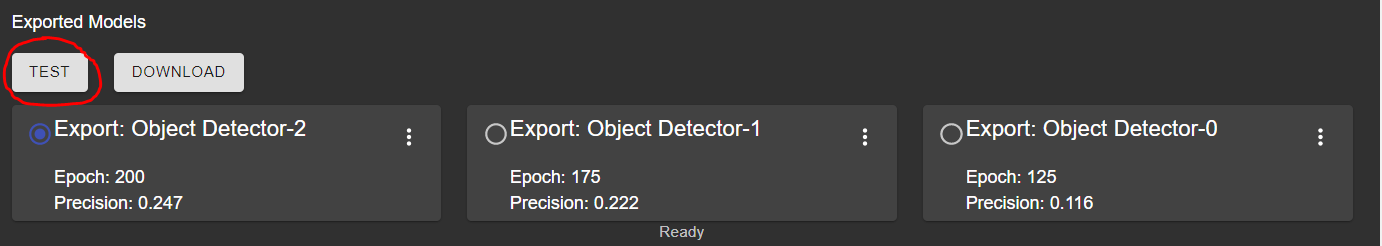
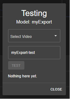
First, click the Select Video box, and click the + that will appear to upload a video.
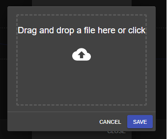
This will open a window that allows you to upload a .mp4 file.
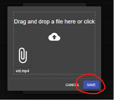
Drop a .mp4 in the dropzone, or click to select the file. Once the file is in the dropzone, click Save.
When uploaded, you will see the video in the dropdown menu, allowing you to select it for the test.
You have the option to change the name of the annotated output video produced by the test.
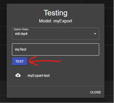
Click the Test button, and you will see the test begin.
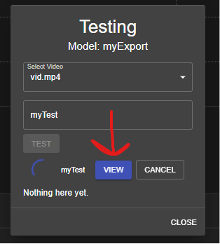
The test uses your model to annotate the video, creating a stream for you to watch as it happens. Click the View button, and the stream will open in a separate tab.
When the test completes, you will see it at the bottom of the test dialog.
You can download the annotated video. Click the download icon next to the test’s name, and your browser will begin the download. The video is currently a .mp4 within a .zip.
Inferencing on a Raspberry Pi
Hardware Requirements
This section requires a Romi or a Raspberry Pi that is running the WPILibPi Image.
Instructions to setup WPILibPi can be found here.
Other hardware that is required is:
A USB Camera
A Coral TPU (Highly Recommended)
Note
A Coral Edge TPU is a USB Accelerator that the Raspberry Pi uses as a co-processor to improve its performance while inferencing. In our experience it has shown to improve performance by around 9 times.
Uploading the Model to the Pi
To upload your tflite model to the Raspberry Pi, you must connect to it and open the Web-interface. Select the Application tab, go to the File Upload section and turn the Extract slider on.
Once this is checked, you can upload the zip that you downloaded from Axon onto the Pi.
Inferencing
Once the model has been uploaded, now the Pi needs python code to utilize it. Here is a link to the provided inference script through the release page: Github
Once this is downloaded, utilize the Vision Application Configuration section to upload the python file.
Once uploaded, utilize the Vision Status tab to check on the state of the script. You should be able to see an update with a framerate indicating that everything is working.
Head to the Vision Settings tab. First click on the camera stream and change the resolution to be greater than 300 pixels by 300 pixels (e.g. 640 by 480).
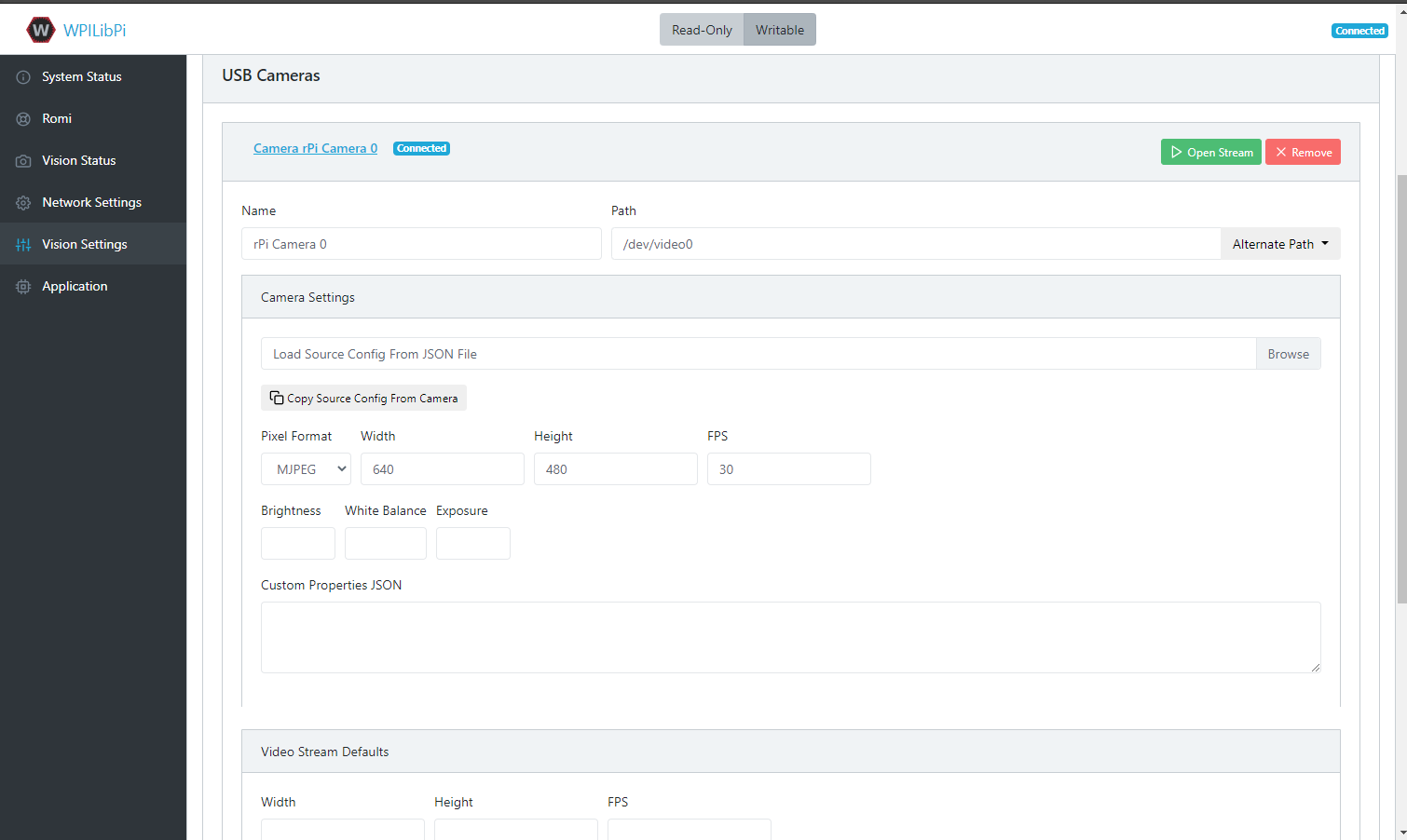
Then click on Open Stream to view the camera stream. Increase the port number at the top by one each time to move through the various camera streams until you arrive at the desired one. The default port is always at 1181, and the additional streams will start at 1182.
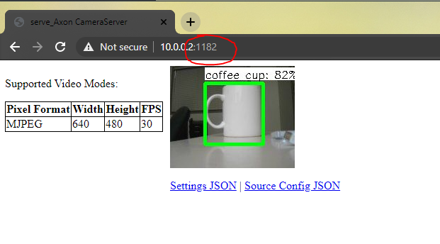
Then you can see the output stream from the Machine Learning Model. You should be able to see the Raspberry Pi identifying objects!
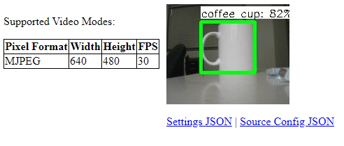
Network Tables
Note
When using a Romi, robot code must be running on the simulator to receive network tables data.
The python script from the releases page that is responsible for inferencing, also pushes that data to network tables. To see the results, one can use the OutlineViewer tool.
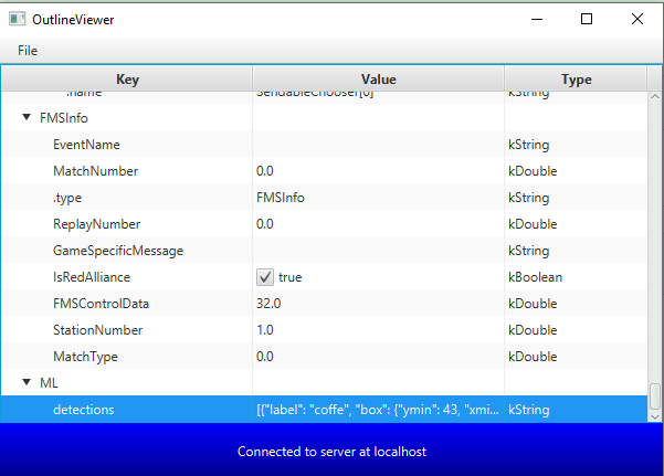
Note
Use Server Location localhost when running on a Romi
Using Inference Output on a Robot
The provided script for running inference on a coprocessor outputs all inference data over NetworkTables for ease of access.
Output Format
Because there can be any number of detected objects in a given image, the inference data is sent in a JSON string to the ML/detections NetworkTables entry. By compiling all data into a single entry, it is certain that the labels match with the bounding boxes, which may not be true if these items were separate entries.
The JSON string has the following format:
[
{
"label": "blue robot",
"box": {
"ymin": 25,
"xmin": 10,
"ymax": 100,
"xmax": 150
},
"confidence": 0.75
},
{
"label": "red robot",
"box": {
"ymin": 111,
"xmin": 163,
"ymax": 240,
"xmax": 320
},
"confidence": 0.99
}
]
The example above shows the value of the ML/detections entry if two objects are detected. It is a list of objects, where the label attribute means the kind of object that was detected. The box attribute describes the bottom left and top right corners of the bounding box, i.e. the box that completely surrounds the detected object within the image. There will be an empty list if no objects are detected. The confidence attribute is how confident the model is that the given object is correctly detected.
There are three more NetworkTables entries that the provided script uses to help the programmer. The first is ML/fps, which tells the programmer how many frames their model is processing per second. Another is ML/coral, which tells the programmer is a Google Coral USB accelerator is currently being used. This is included in case someone removes the Coral from the robot and forgets to put it back, or a similar scenario. The final NetworkTables entry is ML/resolution, which is the string WIDTH, HEIGHT, telling the programmer the size of the processed image, for use with calculations.
Applications of Inference
Machine learning is applicable to the FIRST Robotics Competition when non-uniform objects need to be detected, i.e. a hatch panel from the 2019 game.
A model could also be trained to recognize other robots, if a collision-avoidance system were wanted to be implemented. The WPILib team has found that uniform objects, such as the 2020 Power Cells, are also easily detected by neural networks, but other algorithms may be more appropriate.
Vision Processing
Vision Introduction
What is Vision?
Vision in FRC® uses a camera connected to the robot in order to help teams score and drive, during both the autonomous and teleoperated periods.
Vision Methods
There are two main method that most teams use for vision in FRC.
Streaming
This method involves streaming the camera to the Driver Station so that the driver and manipulator can get visual information from the robot’s point of view. This method is simple and takes little time to implement, making it a good option if you do not need features of vision processing.
Processing
Instead of only streaming the camera to the Driver Station, this method involves using the frames captured by the camera to compute information, such as a game piece’s or target’s angle and distance from the camera. This method requires more technical knowledge and time in order to implement, as well as being more computationally expensive. However, this method can help improve autonomous performance and assist in “auto-scoring” operations during the teleoperated period. This method can be done using the roboRIO or a coprocessor such as the Raspberry Pi using either OpenCV or programs such as GRIP.
For additional information on the pros and cons of using a coprocessor for vision processing, see the next page, Strategies for Vision Programming.
Strategies for Vision Programming
Using computer vision is a great way of making your robot be responsive to the elements on the field and make it much more autonomous. Often in FRC® games there are bonus points for autonomously shooting balls or other game pieces into goals or navigating to locations on the field. Computer vision is a great way of solving many of these problems. And if you have autonomous code that can do the challenge, then it can be used during the teleop period as well to help the human drivers.
There are many options for choosing the components for vision processing and where the vision program should run. WPILib and associated tools support a number of options and give teams a lot of flexibility to decide what to do. This article will attempt to give you some insight into many of the choices and tradeoffs that are available.

OpenCV Computer Vision Library
OpenCV is an open source computer vision library that is widely used throughout academia and industry. It has support from hardware manufactures providing GPU accelerated processing, it has bindings for a number of languages including C++, Java, and Python. It is also well documented with many web sites, books, videos, and training courses so there are lots of resources available to help learn how to use it. The C++ and Java versions of WPILib include the OpenCV libraries, there is support in the library for capturing, processing and viewing video, and tools to help you create your vision algorithms. For more information about OpenCV see https://opencv.org.
Vision Code on roboRIO

Vision code can be embedded into the main robot program on the roboRIO. Building and running the vision code is straightforward because it is built and deployed along with the robot program. The vision code can be written by hand or generated by GRIP in either C++ or Java. The disadvantage of this approach is that having vision code running on the same processor as the robot program can cause performance issues. This is something you will have to evaluate depending on the requirements for your robot and vision program.
In this approach, the vision code simply produces results that the robot code directly uses. Be careful about synchronization issues when writing robot code that is getting values from a vision thread. The GRIP generated code and the VisionRunner class in WPILib make this easier.
Using functions provided by the CameraServer class, the video stream can be sent to dashboards such as Shuffleboard so operators can see what the camera sees. In addition, annotations can be added to the images using OpenCV commands so targets or other interesting objects can be identified in the dashboard view.
Vision Code on DS Computer

When vision code is running on the DS computer, the video is streamed back to the Driver Station laptop for processing. Even the older Classmate laptops are substantially faster at vision processing than the roboRIO. GRIP can be run on the Driver Station laptop directly with the results sent back to the robot using NetworkTables. Alternatively you can write your own vision program using a language of your choosing. Python makes a good choice since there is a native NetworkTables implementation and the OpenCV bindings are very good.
After the images are processed, the key values such as the target position, distance or anything else you need can be sent back to the robot with NetworkTables. This approach generally has higher latency, as delay is added due to the images needing to be sent to the laptop. Bandwidth limitations also limit the maximum resolution and FPS of the images used for processing.
The video stream can be displayed on Shuffleboard or in GRIP.
Vision Code on Coprocessor

Coprocessors such as the Raspberry Pi are ideal for supporting vision code (see Using the Raspberry Pi for FRC). The advantage is that they can run full speed and not interfere with the robot program. In this case, the camera is probably connected to the coprocessor or (in the case of Ethernet cameras) an Ethernet switch on the robot. The program can be written in any language; Python is a good choice because of its simple bindings to OpenCV and NetworkTables. Some teams have used high performance vision coprocessors such as the Nvidia Jetson for fastest speed and highest resolution, although this approach generally requires advanced Linux and programming knowledge.
This approach takes a bit more programming expertise as well as a small amount of additional weight, but otherwise it brings the best of both worlds compared to the other two approaches, as coprocessors are much faster than the roboRIO and the image processing can be performed with minimal latency or bandwidth use.
Data can be sent from the vision program on the coprocessor to the robot using NetworkTables or a private protocol over a network or serial connection.
Camera Options
There are a number of camera options supported by WPILib. Cameras have a number of parameters that affect operation; for example, frame rate and image resolution affect the quality of the received images, but when set too high impact processing time and, if sent to the driver station, may exceed the available bandwidth on the field.
The CameraServer class in C++ and Java is used to interface with cameras connected to the robot. It retrieve frames for local processing through a Source object and sends the stream to your driver station for viewing or processing there.
Target Info and Retroreflection
Many FRC® games have retroreflective tape attached to field elements to aid in vision processing. This document describes the Vision Targets from the 2016 FRC game and the visual properties of the material making up the targets.
Note
For official dimensions and drawings of all field components, please see the Official Field Drawings.
Targets
Each 2016 vision target consists of a 1’ 8” wide, 1’ tall U-shape made of 2” wide retroreflective material (3M 8830 Silver Marking Film). The targets are located immediately adjacent to the bottom of each high goal. When properly lit, the retroreflective tape produces a bright and/or color-saturated marker.
Retroreflectivity vs. Reflectivity

Highly reflective materials are generally mirrored so that light “bounces off” at a supplementary angle. As shown above-left, the blue and red angles sum to 180 degrees. An equivalent explanation is that the light reflects about the surface normal the green line drawn perpendicular to the surface. Notice that a light pointed at the surface will return to the light source only if the blue angle is ~90 degrees.
Retro-reflective materials are not mirrored, but it will typically have either shiny facets across the surface, or it will have a pearl-like appearance. Not all faceted or pearl-like materials are retro-reflective, however. Retro-reflective materials return the majority of light back to the light source, and they do this for a wide range of angles between the surface and the light source, not just the 90 degree case. Retro-reflective materials accomplish this using small prisms, such as found on a bicycle or roadside reflector, or by using small spheres with the appropriate index of refraction that accomplish multiple internal reflections. In nature, the eyes of some animals, including house cats, also exhibit the retro-reflective effect typically referred to as night-shine. The Wikipedia article on retroreflectors goes into more detail on how retro-reflection is accomplished.
Examples of Retroreflection

This material should be relatively familiar as it is often used to enhance nighttime visibility of road signs, bicycles, and pedestrians.
Initially, retro-reflection may not seem like a useful property for nighttime safety, but when the light and eye are near one another, as shown above, the reflected light returns to the eye, and the material shines brightly even at large distances. Due to the small angle between the driver’s eyes and vehicle headlights, retro-reflective materials can greatly increase visibility of distant objects during nighttime driving.
Demonstration
To further explore retro-reflective material properties:
Place a piece of the material on a wall or vertical surface
Stand 10-20 feet away, and shine a small flashlight at the material.
Start with the light held at your belly button, and raise it slowly until it is between your eyes. As the light nears your eyes, the intensity of the returned light will increase rapidly.
Alter the angle by moving to other locations in the room and repeating. The bright reflection should occur over a wide range of viewing angles, but the angle from light source to eye is key and must be quite small.
Experiment with different light sources. The material is hundreds of times more reflective than white paint; so dim light sources will work fine. For example, a red bicycle safety light will demonstrate that the color of the light source determines the color of the reflected light. If possible, position several team members at different locations, each with their own light source. This will show that the effects are largely independent, and the material can simultaneously appear different colors to various team members. This also demonstrates that the material is largely immune to environmental lighting. The light returning to the viewer is almost entirely determined by a light source they control or one directly behind them. Using the flashlight, identify other retro-reflective articles already in your environment: on clothing, backpacks, shoes, etc.
Lighting
We have seen that the retro-reflective tape will not shine unless a light source is directed at it, and the light source must pass very near the camera lens or the observer’s eyes. While there are a number of ways to accomplish this, a very useful type of light source to investigate is the ring flash, or ring light, shown above. It places the light source directly on or around the camera lens and provides very even lighting. Because of their bright output and small size, LEDs are particularly useful for constructing this type of device.
As shown above, inexpensive circular arrangements of LEDs are available in a variety of colors and sizes and are easy to attach to cameras, and some can even be powered off of a Raspberry Pi. While not designed for diffuse even lighting, they work quite well for causing retro-reflective tape to shine. A small green LED ring is available through FIRST Choice. Other similar LED rings are available from suppliers such as SuperBrightLEDs.
Sample Images
Sample images are located with the code examples for each language (packaged with LabVIEW, and in a separate ZIP in the same location as the C++/Java samples).
Identifying and Processing the Targets
Once an image is captured, the next step is to identify Vision Target(s) in the image. This document will walk through one approach to identifying the 2016 targets. Note that the images used in this section were taken with the camera intentionally set to underexpose the images, producing very dark images with the exception of the lit targets, see the section on Camera Settings for details.
Additional Options
This document walks through the approach used by the example code provided in LabVIEW (for PC or roboRIO), C++ and Java. In addition to these options teams should be aware of the following alternatives that allow for vision processing on the Driver Station PC or an on-board PC:
Original Image
The image shown below is the starting image for the example described here. The image was taken using the green ring light available in FIRST® Choice combined with an additional ring light of a different size. Additional sample images are provided with the vision code examples.

What is HSL/HSV?
The Hue or tone of the color is commonly seen on the artist’s color wheel and contains the colors of the rainbow Red, Orange, Yellow, Green, Blue, Indigo, and Violet. The hue is specified using a radial angle on the wheel, but in imaging the circle typically contains only 256 units, starting with red at zero, cycling through the rainbow, and wrapping back to red at the upper end. Saturation of a color specifies amount of color, or the ratio of the hue color to a shade of gray. Higher ratio means more colorful, less gray. Zero saturation has no hue and is completely gray. Luminance or Value indicates the shade of gray that the hue is blended with. Black is 0 and white is 255.
The example code uses the HSV color space to specify the color of the target. The primary reason is that it readily allows for using the brightness of the targets relative to the rest of the image as a filtering criteria by using the Value (HSV) or Luminance (HSL) component. Another reason to use the HSV color system is that the thresholding operation used in the example runs more efficiently on the roboRIO when done in the HSV color space.
Masking
In this initial step, pixel values are compared to constant color or brightness values to create a binary mask shown below in yellow. This single step eliminates most of the pixels that are not part of a target’s retro-reflective tape. Color based masking works well provided the color is relatively saturated, bright, and consistent. Color inequalities are generally more accurate when specified using the HSL (Hue, Saturation, and Luminance) or HSV (Hue, Saturation, and Value) color space than the RGB (Red, Green, and Blue) space. This is especially true when the color range is quite large in one or more dimension.
Notice that in addition to the target, other bright parts of the image (overhead light and tower lighting) are also caught by the masking step.
Particle Analysis
After the masking operation, a particle report operation is used to examine the area, bounding rectangle, and equivalent rectangle for the particles. These are used to compute several scored terms to help pick the shapes that are most rectangular. Each test described below generates a score (0-100) which is then compared to pre-defined score limits to decide if the particle is a target or not.
Coverage Area
The Area score is calculated by comparing the area of the particle compared to the area of the bounding box drawn around the particle. The area of the retroreflective strips is 80 square inches (~516 \(cm^2\)). The area of the rectangle that contains the target is 240 square inches (~0.15 \(m^2\)). This means that the ideal ratio between area and bounding box area is 1/3. Area ratios close to 1/3 will produce a score near 100, as the ratio diverges from 1/3 the score will approach 0.
Aspect Ratio
The aspect ratio score is based on (Particle Width / Particle Height). The width and height of the particle are determined using something called the “equivalent rectangle”. The equivalent rectangle is the rectangle with side lengths \(x\) and \(y\) where \(2x+2y\) equals the particle perimeter and \(x \cdot y\) equals the particle area. The equivalent rectangle is used for the aspect ratio calculation as it is less affected by skewing of the rectangle than using the bounding box. When using the bounding box rectangle for aspect ratio, as the rectangle is skewed the height increases and the width decreases.
The target is 20” (508 mm) wide by 12” (304.8 mm) tall, for a ratio of 1.6. The detected aspect ratio is compared to this ideal ratio. The aspect ratio score is normalized to return 100 when the ratio matches the target ratio and drops linearly as the ratio varies below or above.
Moment
The moment measurement calculates the particles moment of inertia about it’s center of mass. This measurement provides a representation of the pixel distribution in the particle. The ideal score for this test is ~0.28. See: Moment of Inertia
X/Y Profiles
The edge score describes whether the particle matches the appropriate profile in both the X and Y directions. As shown, it is calculated using the row and column averages across the bounding box extracted from the original image and comparing that to a profile mask. The score ranges from 0 to 100 based on the number of values within the row or column averages that are between the upper and lower limit values.
Measurements
If a particle scores well enough to be considered a target, it makes sense to calculate some real-world measurements such as position and distance. The example code includes these basic measurements, so let’s look at the math involved to better understand it.
Position
The target position is well described by both the particle and the bounding box, but all coordinates are in pixels with 0,0 being at the top left of the screen and the right and bottom edges determined by the camera resolution. This is a useful system for pixel math, but not nearly as useful for driving a robot; so let’s change it to something that may be more useful.
To convert a point from the pixel system to the aiming system, we can use the formula shown below.
The resulting coordinates are close to what you may want, but the Y axis is inverted. This could be corrected by multiplying the point by [1,-1] (Note: this is not done in the sample code). This coordinate system is useful because it has a centered origin and the scale is similar to joystick outputs and Drive inputs.
Field of View
You can use known constants and the position of the target on the coordinate plane to determine your distance, yaw, and pitch from the target. However, in order to calculate these, you must determine your FOV (field of view). In order to empirically determine vertical field of view, set your camera a set distance away from an flat surface, and measure the distance between the topmost and bottommost row of pixels.
You can find the horizontal FOV using the same method, but using the distance between the first and last column of pixels.
Pitch and Yaw
Finding the pitch and yaw of the target relative to your robot is simple once you know your FOVs and the location of your target in the aiming coordinate system.
Distance
If your target is at a significantly different height than your robot, you can use known constants, such as the physical height of the target and your camera, as well as the angle your camera is mounted, to calculate the distance between your camera and the target.
Another option is to create a lookup table for area to distance, or to estimate the inverse variation constant of area and distance. However, this method is less accurate.
Note
For best results for the above methods of estimating angle and distance, you can calibrate your camera using OpenCV to get rid of any distortions that may be affecting accuracy by reprojecting the pixels of the target using the calibration matrix.
Read and Process Video: CameraServer Class
Concepts
The cameras typically used in FRC® (commodity USB and Ethernet cameras such as the Axis camera) offer relatively limited modes of operation. In general, they provide only a single image output (typically in an RGB compressed format such as JPG) at a single resolution and frame rate. USB cameras are particularly limited as only one application may access the camera at a time.
CameraServer supports multiple cameras. It handles details such as automatically reconnecting when a camera is disconnected, and also makes images from the camera available to multiple “clients” (e.g. both your robot code and the dashboard can connect to the camera simultaneously).
Camera Names
Each camera in CameraServer must be uniquely named. This is also the name that appears for the camera in the Dashboard. Some variants of the CameraServer startAutomaticCapture() and addAxisCamera() functions will automatically name the camera (e.g. “USB Camera 0” or “Axis Camera”), or you can give the camera a more descriptive name (e.g. “Intake Cam”). The only requirement is that each camera have a unique name.
USB Camera Notes
CPU Usage
The CameraServer is designed to minimize CPU usage by only performing compression and decompression operations when required and automatically disabling streaming when no clients are connected.
To minimize CPU usage, the dashboard resolution should be set to the same resolution as the camera; this allows the CameraServer to not decompress and recompress the image, instead, it can simply forward the JPEG image received from the camera directly to the dashboard. It’s important to note that changing the resolution on the dashboard does not change the camera resolution; changing the camera resolution may be done by calling setResolution() on the camera object.
USB Bandwidth
The roboRIO can only transmit and receive so much data at a time over its USB interfaces. Camera images can require a lot of data, and so it is relatively easy to run into this limit. The most common cause of a USB bandwidth error is selecting a non-JPEG video mode or running too high of a resolution, particularly when multiple cameras are connected.
Architecture
The CameraServer consists of two layers, the high level WPILib CameraServer class and the low level cscore library.
CameraServer Class
The CameraServer class (part of WPILib) provides a high level interface for adding cameras to your robot code. It also is responsible for publishing information about the cameras and camera servers to NetworkTables so that Driver Station dashboards such as the LabVIEW Dashboard and Shuffleboard can list the cameras and determine where their streams are located. It uses a singleton pattern to maintain a database of all created cameras and servers.
Some key functions in CameraServer are:
startAutomaticCapture(): Add a USB camera (e.g. Microsoft LifeCam) and starts a server for it so it can be viewed from the dashboard.addAxisCamera(): Add an Axis camera. Even if you aren’t processing images from the Axis camera in your robot code, you may want to use this function so that the Axis camera appears in the Dashboard’s drop down list of cameras. It also starts a server so the Axis stream can still be viewed when your driver station is connected to the roboRIO via USB (useful at competition if you have both the Axis camera and roboRIO connected to the two robot radio Ethernet ports).getVideo(): Get OpenCV access to a camera. This allows you to get images from the camera for image processing on the roboRIO (in your robot code).putVideo(): Start a server that you can feed OpenCV images to. This allows you to pass custom processed and/or annotated images to the dashboard.
cscore Library
The cscore library provides the lower level implementation to:
Get images from USB and HTTP (e.g. Axis) cameras
Change camera settings (e.g. contrast and brightness)
Change camera video modes (pixel format, resolution and frame rate)
Act as a web server and serve images as a standard MJPEG stream
Convert images to/from OpenCV
Matobjects for image processing
Sources and Sinks
The basic architecture of the cscore library is similar to that of MJPGStreamer, with functionality split between sources and sinks. There can be multiple sources and multiple sinks created and operating simultaneously.
An object that generates images is a source and an object that accepts/consumes images is a sink. The generate/consume is from the perspective of the library. Thus cameras are sources (they generate images). The MJPEG web server is a sink because it accepts images from within the program (even though it may be forwarding those images on to a web browser or dashboard). Sources may be connected to multiple sinks, but sinks can be connected to one and only one source. When a sink is connected to a source, the cscore library takes care of passing each image from the source to the sink.
Sources obtain individual frames (such as provided by a USB camera) and fire an event when a new frame is available. If no sinks are listening to a particular source, the library may pause or disconnect from a source to save processor and I/O resources. The library autonomously handles camera disconnects/reconnects by simply pausing and resuming firing of events (e.g. a disconnect results in no new frames, not an error).
Sinks listen to a particular source’s event, grab the latest image, and forward it to its destination in the appropriate format. Similarly to sources, if a particular sink is inactive (e.g. no client is connected to a configured MJPEG over HTTP server), the library may disable parts of its processing to save processor resources.
User code (such as that used in a FRC robot program) can act as either a source (providing processed frames as if it were a camera) or as a sink (receiving a frame for processing) via OpenCV source and sink objects. Thus an image processing pipeline that gets images from a camera and serves the processed images out looks like the below graph:

Because sources can have multiple sinks connected, the pipeline may branch. For example, the original camera image can also be served by connecting the UsbCamera source to a second MjpegServer sink in addition to the CvSink, resulting in the below graph:

When a new image is captured by the camera, both the CvSink and the MjpegServer [1] receive it.
The above graph is what the following CameraServer snippet creates:
import edu.wpi.first.cameraserver.CameraServer;
import edu.wpi.cscore.CvSink;
import edu.wpi.cscore.CvSource;
// Creates UsbCamera and MjpegServer [1] and connects them
CameraServer.startAutomaticCapture();
// Creates the CvSink and connects it to the UsbCamera
CvSink cvSink = CameraServer.getVideo();
// Creates the CvSource and MjpegServer [2] and connects them
CvSource outputStream = CameraServer.putVideo("Blur", 640, 480);
#include "cameraserver/CameraServer.h"
// Creates UsbCamera and MjpegServer [1] and connects them
frc::CameraServer::StartAutomaticCapture();
// Creates the CvSink and connects it to the UsbCamera
cs::CvSink cvSink = frc::CameraServer::GetVideo();
// Creates the CvSource and MjpegServer [2] and connects them
cs::CvSource outputStream = frc::CameraServer::PutVideo("Blur", 640, 480);
The CameraServer implementation effectively does the following at the cscore level (for explanation purposes). CameraServer takes care of many of the details such as creating unique names for all cscore objects and automatically selecting port numbers. CameraServer also keeps a singleton registry of created objects so they aren’t destroyed if they go out of scope.
import edu.wpi.cscore.CvSink;
import edu.wpi.cscore.CvSource;
import edu.wpi.cscore.MjpegServer;
import edu.wpi.cscore.UsbCamera;
// Creates UsbCamera and MjpegServer [1] and connects them
UsbCamera usbCamera = new UsbCamera("USB Camera 0", 0);
MjpegServer mjpegServer1 = new MjpegServer("serve_USB Camera 0", 1181);
mjpegServer1.setSource(usbCamera);
// Creates the CvSink and connects it to the UsbCamera
CvSink cvSink = new CvSink("opencv_USB Camera 0");
cvSink.setSource(usbCamera);
// Creates the CvSource and MjpegServer [2] and connects them
CvSource outputStream = new CvSource("Blur", PixelFormat.kMJPEG, 640, 480, 30);
MjpegServer mjpegServer2 = new MjpegServer("serve_Blur", 1182);
mjpegServer2.setSource(outputStream);
#include "cscore_oo.h"
// Creates UsbCamera and MjpegServer [1] and connects them
cs::UsbCamera usbCamera("USB Camera 0", 0);
cs::MjpegServer mjpegServer1("serve_USB Camera 0", 1181);
mjpegServer1.SetSource(usbCamera);
// Creates the CvSink and connects it to the UsbCamera
cs::CvSink cvSink("opencv_USB Camera 0");
cvSink.SetSource(usbCamera);
// Creates the CvSource and MjpegServer [2] and connects them
cs::CvSource outputStream("Blur", cs::PixelFormat::kMJPEG, 640, 480, 30);
cs::MjpegServer mjpegServer2("serve_Blur", 1182);
mjpegServer2.SetSource(outputStream);
Reference Counting
All cscore objects are internally reference counted. Connecting a sink to a source increments the source’s reference count, so it’s only strictly necessary to keep the sink in scope. The CameraServer class keeps a registry of all objects created with CameraServer functions, so sources and sinks created in that way effectively never go out of scope (unless explicitly removed).
2017 Vision Examples
LabVIEW
The 2017 LabVIEW Vision Example is included with the other LabVIEW examples. From the Splash screen, click Support->Find FRC® Examples or from any other LabVIEW window, click Help->Find Examples and locate the Vision folder to find the 2017 Vision Example. The example images are bundled with the example.
C++/Java
We have provided a GRIP project and the description below, as well as the example images, bundled into a ZIP that can be found on TeamForge.
See Using Generated Code in a Robot Program for details about integrating GRIP generated code in your robot program.
The code generated by the included GRIP project will find OpenCV contours for green particles in images like the ones included in the Vision Images folder of this ZIP. From there you may wish to further process these contours to assess if they are the target. To do this:
Use the boundingRect method to draw bounding rectangles around the contours
The LabVIEW example code calculates 5 separate ratios for the target. Each of these ratios should nominally equal 1.0. To do this, it sorts the contours by size, then starting with the largest, calculates these values for every possible pair of contours that may be the target, and stops if it finds a target or returns the best pair it found.
In the formulas below, each letter refers to a coordinate of the bounding rect (H = Height, L = Left, T = Top, B = Bottom, W = Width) and the numeric subscript refers to the contour number (1 is the largest contour, 2 is the second largest, etc).
Top height should be 40% of total height (4 in / 10 in):
Top of bottom stripe to top of top stripe should be 60% of total height (6 in / 10 in):
The distance between the left edge of contour 1 and the left edge of contour 2 should be small relative to the width of the 1st contour; then we add 1 to make the ratio centered on 1:
The widths of both contours should be about the same:
The larger stripe should be twice as tall as the smaller one
Each of these ratios is then turned into a 0-100 score by calculating:
To determine distance, measure pixels from top of top bounding box to bottom of bottom bounding box:
The LabVIEW example uses height as the edges of the round target are the most prone to noise in detection (as the angle points further from the camera the color looks less green). The downside of this is that the pixel height of the target in the image is affected by perspective distortion from the angle of the camera. Possible fixes include:
Try using width instead
Empirically measure height at various distances and create a lookup table or regression function
Mount the camera to a servo, center the target vertically in the image and use servo angle for distance calculation (you’ll have to work out the proper trig yourself or find a math teacher to help!)
Correct for the perspective distortion using OpenCV. To do this you will need to calibrate your camera with OpenCV. This will result in a distortion matrix and camera matrix. You will take these two matrices and use them with the undistortPoints function to map the points you want to measure for the distance calculation to the “correct” coordinates (this is much less CPU intensive than undistorting the whole image)
Vision with WPILibPi
A Video Walkthrough of using WPILibPi with the Raspberry Pi
Note
The video mentions FRCVision which is the old name of WPILibPi.
At the “RSN Spring Conference, Presented by WPI” in 2020, Peter Johnson from the WPILib team gave a presentation on FRC® Vision with a Raspberry Pi.
The link to the presentation is available here.
Using a Coprocessor for vision processing
Vision processing using libraries like OpenCV for recognizing field targets or game pieces can often be a CPU intensive process. Often the load isn’t too significant and the processing can easily be handled by the roboRIO. In cases where there are more camera streams or the image processing is complex, it is desirable to off-load the roboRIO by putting the code and the camera connection on a different processor. There are a number of choices of processors that are popular in FRC® such as the Raspberry PI, the intel-based Kangaroo, the LimeLight for the ultimate in simplicity, or for more complex vision code a graphics accelerator such as one of the nVidia Jetson models.
Strategy
Generally the idea is to set up the coprocessor with the required software that generally includes:
OpenCV - the open source computer vision library
NetworkTables - to commute the results of the image processing to the roboRIO program
Camera server library - to handle the camera connections and publish streams that can be viewed on a dashboard
The language library for whatever computer language is used for the vision program
The actual vision program that does the object detection
The coprocessor is connected to the roboRIO network by plugging it into the extra ethernet port on the network router or, for more connections, adding a small network switch to the robot. The cameras are plugged into the coprocessor, it acquires the images, processes them, and publishes the results, usually target location information, to NetworkTables so it is can be consumed by the robot program for steering and aiming.

Streaming camera data to the dashboard
It is often desirable to simply stream the camera data to the dashboard over the robot network. In this case one or more camera connections can be sent to the network and viewed on a dashboard such as Shuffleboard or a web browser. Using Shuffleboard has the advantage of having easy controls to set the camera resolution and bit rate as well as integrating the camera streams with other data sent from the robot.
It is also possible to process images and add annotation to the image, such as target lines or boxes showing what the image processing code has detected then send it forward to the dashboard to make it easier for operators to see a clear picture of what’s around the robot.
Using the Raspberry Pi for FRC
One of the most popular coprocessor choices is the Raspberry Pi because:
Low cost - around $35
High availability - it’s easy to find Raspberry Pis from a number of suppliers, including Amazon
Very good performance - the current Raspberry Pi 3b+ has the following specifications:
Technical Specifications: - Broadcom BCM2837BO 64 bit ARMv8 QUAD Core A53 64bit Processor powered Single Board Computer run at 1.4GHz - 1GB RAM - BCM43143 WiFi on board - Bluetooth Low Energy (BLE) on board - 40 pin extended GPIO - 4 x USB2 ports - 4 pole Stereo output and Composite video port - Full size HDMI - CSI camera port for connecting the Raspberry - Pi camera - DSI display port for connecting the Raspberry - Pi touch screen display - MicroSD port for loading your operating system and storing data - Upgraded switched Micro USB power source (now supports up to 2.5 Amps.
Pre-built Raspberry Pi image
To make using the Raspberry Pi as easy as possible for teams, there is a provided Raspberry Pi image. The image can be copied to a micro SD card, inserted into the Pi, and booted. By default it supports:
A web interface for configuring it for the most common functions
Supports an arbitrary number camera streams (defaults to one) that are published on the network interface
OpenCV, NetworkTables, Camera Server, and language libraries for C++, Java, and Python custom programs
If the only requirement is to stream one or more cameras to the network (and dashboard) then no programming is required and can be completely set up through the web interface.
The next section discusses how to install the image onto a flash card and boot the Pi.
What you need to get the Pi image running
To start using the Raspberry Pi as a video or image coprocessor you need the following:
A Raspberry Pi 3 B, Raspberry Pi 3 B+, or a Raspberry Pi 4 B
A micro SD card that is at least 8 GB to hold all the provided software, with a recommended Speed Class of 10 (10MB/s)
An ethernet cable to connect the Pi to your roboRIO network
A USB micro power cable to connect to the Voltage Regulator Module (VRM) on your robot. It is recommended to use the VRM connection for power rather than powering it from one of the roboRIO USB ports for higher reliability
A laptop that can write the MicroSD card, either using a USB dongle (preferred) or a SD to MicroSD adapter that ships with most MicroSD cards
Shown is an inexpensive USB dongle that will write the FRC® image to the MicroSD card.
Installing the image to your MicroSD card
Getting the FRC Raspberry PI image
The image is stored on the GitHub release page for the WPILibPi repository.
In addition to the instructions on this page, see the documentation on the GitHub web page (below).
The image is fairly large so have a fast internet connection when downloading it. Always use the most recent release from the top of the list of releases.
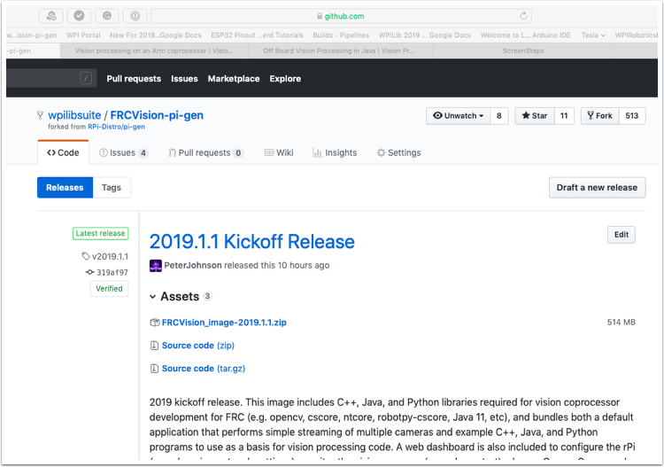
Copy the image to your MicroSD card
Download and install Etcher to image the micro SD card. The micro SD card needs to be at least 8 GB. A micro SD to USB dongle works well for writing to micro SD cards.
Flash the MicroSD card with the image using Etcher by selecting the zip file as the source, your SD card as the destination and click “Flash”. Expect the process to take about 3 minutes on a fairly fast laptop.
Testing the Raspberry PI
Put the micro SD card in a rPi 3 and apply power.
Connect the rPi 3 ethernet to a LAN or PC. Open a web browser and connect to
http://wpilibpi.local/to open the web dashboard. On the first bootup the filesystem will be writable, but later bootups will default to read only, so it’s necessary to click the “writable” button to make changes.
Logging into the Raspberry PI
Most tasks with the rPi can be done from the web console interface. Sometimes for advanced use such as program development on the rPi it is necessary to log in. To log in, use the default Raspberry PI password:
Username: pi
Password: raspberry
The Raspberry PI
FRC Console
The FRC® image for the Raspberry PI includes a console that can be viewed in any web browser that makes it easy to:
Look at the Raspberry PI status
View the status of the background process running the camera
View or change network settings
Look at each camera plugged into the rPI and add additional cameras
Load a new vision program onto the rPI
Setting the rPI to be Read-Only vs. Writable
The rPI is normally set to Read-Only which means that the file system cannot be changed. This ensures that if power is removed without first shutting down the rPi the file system isn’t corrupted. When settings are changed (following sections), the new settings cannot be saved while the rPI file system is set as Read-Only. Buttons are provided that allow the file system to be changed from Read-Only to Writable and back whenever changes are made. If the other buttons that change information stored on the rPI cannot be press, check the Read-Only status of the system.
Status of the network connection to the rPI
There is a label in the top right corner of the console that indicates if the rPi is currently connected. It will change from Connected to Disconnected if there is no longer a network connection to the rPi.
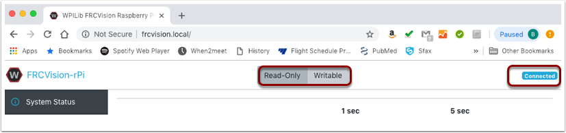
System status
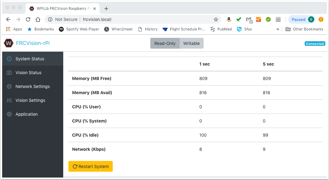
The system status shows what the CPU on the rPI is doing at any time. There are two columns of status values, on being a 1 second average and the other a 5 second average. Shown is:
free and available RAM on the PI
CPU usage for user processes and system processes as well as idle time.
And network bandwidth - which allows one to determine if the used camera bandwidth is exceeding the maximum bandwidth allowed in the robot rules for any year.
Vision Status
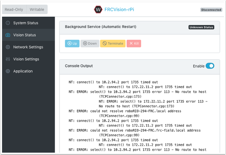
Allows monitoring of the task which is running the camera code in the rPI, either one of the default programs or your own program in Java, C++, or Python. You can also enable and view the console output to see messages coming from the background camera service. In this case there are number of messages about being unable to connect to NetworkTables (NT: connect()) because in this example the rPI is simply connected to a laptop with no NetworkTables server running (usually the roboRIO.)
Network Settings
The rPI network settings have options to connect to the PI:
DHCP - the default name resolution usually used by the roboRIO. The default name is wpilibpi.local.
Static - where a fixed IP address, network mask, and router settings are filled in explicitly
DHCP with Static Fallback - DHCP with Static Fallback - the PI will try to get an IP address via DHCP, but if it can’t find a DHCP server, it will use the provided static IP address and parameters
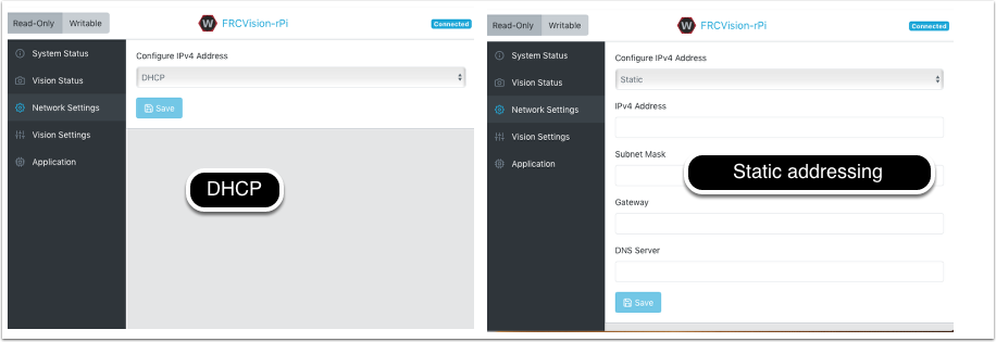
The picture above is showing the settings for both DHCP and Static IP Addressing. The mDNS name for the rPi should always work regardless of the options selected above.
Vision Settings
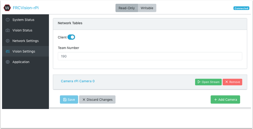
The Vision Settings are to set the parameters for each camera and whether the rPI should be a NetworkTables client or server. There can only be one server on the network and the roboRIO is always a server. Therefor when connected to a roboRIO, the rPI should always be in client mode with the team number filled in. If testing on a desktop setup with no roboRIO or anything acting as a server then it should be set to Server (Client switch is off).
To view and manipulate all the camera settings click on the camera in question. In this case the camera is called “Camera rPi Camera 0” and clicking on the name reveals the current camera view and the associated settings.
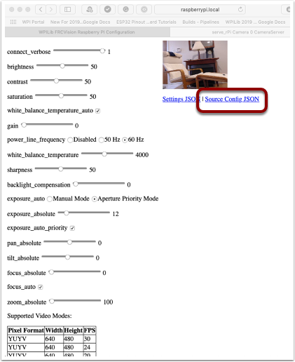
Manipulating the camera settings is reflected in the current camera view. The bottom of the page shows all the possible camera modes (combinations of Width, Height, and frame rates) that are supported by this camera.
Note
If the camera image is not visible on the Open Stream screen then check the supported video modes at the bottom of the page. Then go back to ‘Vision Settings’ and click on the camera in question and verify that the pixel format, width, height, and FPS are listed in the supported video modes.
Getting the current settings to persist over reboots
The rPi will load all the camera settings on startup. Editing the camera configuration in the above screen is temporary. To make the values persist click on the “Load Source Config From Camera” button and the current settings will be filled in on the camera settings fields. Then click “Save” at the bottom of the page. Note: you must set the file system Writeable in order to save the settings. The Writeable button is at the top of the page.
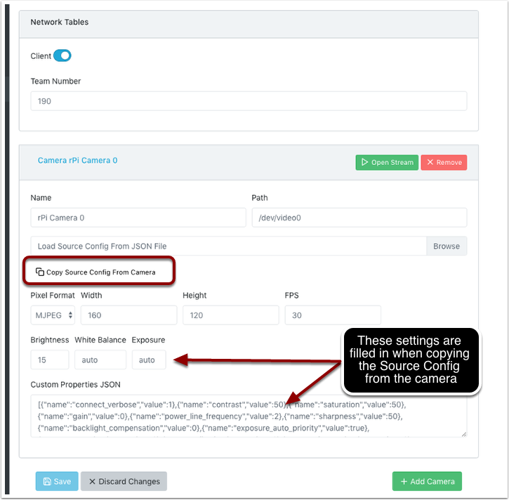
There are some commonly used camera settings values shown in the camera settings (above). These values Brightness, White Balance, and Exposure are loaded into the camera before the user JSON file is applied. So if a user JSON file contains those settings they will overwrite the ones from the text field.
Application
The Application tab shows the application that is currently running on the rPi.
Vision workflows
There is a sample vision program using OpenCV in each of the supported languages, C++, Java, or Python. Each sample program can capture and stream video from the rPi. In addition, the samples have some minimal OpenCV. They are all set up to be extended to replace the provided OpenCV sample code with the code needed for the robot application. The rPi Application tab supports a number of programming workflows:
Stream one or more cameras from the rPi for consumption on the driver station computer and displayed using ShuffleBoard
Edit and build one of the sample programs (one for each language: Java, C++ or Python) on the rPi using the included toolchains
Download a sample program for the chosen language and edit and build it on your development computer. Then upload that built program back to the rPi
Do everything yourself using completely custom applications and scripts (probably based on one of the samples)
The running application can be changed by selecting one of the choices in the drop-down menu. The choices are:
Built-in multi camera streaming which steams whatever cameras are plugged into the rPi. The camera configuration including number of cameras can be set on the “Vision Settings” tab.
Custom application which doesn’t upload anything to the rPi and assumes that the developer wants to have a custom program and script.
Java, C++ or Python pre-installed sample programs that can be edited into your own application.
Java, C++, or Python uploaded program. Java programs require a
.jarfile with the compiled program and C++ programs require an rPi executable to be uploaded to the rPI.
When selecting one of the Upload options, a file chooser is presented where the jar, executable or Python program can be selected and uploaded to the rPi. In the following picture an Uploaded Java jar is chosen and the “Choose File” button will select a file and clicking on the “Save” button will upload the selected file.
Note: in order to Save a new file onto the rPi, the file system has to be set writeable using the “Writable” button at the top left of the web page. After saving the new file, set the file system back to “Read-Only” so that it is protected against accidental changes.
Using CameraServer
Grabbing Frames from CameraServer
The WPILibPi image comes with all the necessary libraries to make your own vision processing system. In order to get the current frame from the camera, you can use the CameraServer library. For information about CameraServer, the Read and Process Video: CameraServer Class.
from cscore import CameraServer
import cv2
import numpy as np
CameraServer.enableLogging()
camera = CameraServer.startAutomaticCapture()
camera.setResolution(width, height)
sink = cs.getVideo()
while True:
time, input_img = cvSink.grabFrame(input_img)
if time == 0: # There is an error
continue
Note
OpenCV reads in the image as BGR, not RGB for historical reasons. Use cv2.cvtColor if you want to change it to RGB.
Below is an example of an image that might be grabbed from CameraServer.
Sending frames to CameraServer
Sometimes, you may want to send processed video frames back to the CameraServer instance for debugging purposes, or viewing in a dashboard application like Shuffleboard.
#
# CameraServer initialization code here
#
output = cs.putVideo("Name", width, height)
while True:
time, input_img = cvSink.grabFrame(input_img)
if time == 0: # There is an error
output.notifyError(sink.getError())
continue
#
# Insert processing code here
#
output.putFrame(processed_img)
As an example, the processing code could outline the target in red, and show the corners in yellow for debugging purposes.
Below is an example of a fully processed image that would be sent back to CameraServer and displayed on the Driver Station computer.
Thresholding an Image
In order to turn a colored image, such as the one captured by your camera, into a binary image, with the target as the “foreground”, we need to threshold the image using the hue, saturation, and value of each pixel.
The HSV Model
Unlike RGB, HSV allows you to not only filter based on the colors of the pixels, but also by the intensity of color and the brightness.
Hue: Measures the color of the pixel.
Saturation: Measures the intensity of color of the pixel.
Value: Measures the brighness of the pixel.
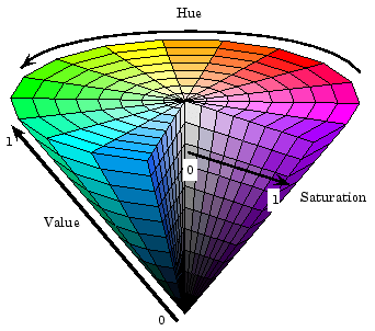
You can use OpenCV to convert a BGR image matrix to HSV.
hsv_img = cv2.cvtColor(input_img, cv2.COLOR_BGR2HSV)
Note
OpenCV’s hue range is from 1° to 180° instead of the common 1° to 360°. In order to convert a common hue value to OpenCV, divide by 2.
Thresholding
We will use this field image as an example for the whole process of image processing.
By thresholding the image using HSV, you can separate the image into the vision target (foreground), and the other things that the camera sees (background). The following code example converts a HSV image into a binary image by thresholding with HSV values.
binary_img = cv2.inRange(hsv_img, (min_hue, min_sat, min_val), (max_hue, max_sat, max_val))
Note
These values may have to be tuned on an per-venue basis, as ambient lighting may differ across venues. It is recommended to allow editing of these values through NetworkTables in order to facilitate on-the-fly editing.
After thresholding, your image should look like this.

As you can see, the thresholding process may not be 100% clean. You can use morphological operations to deal with the noise.
Morphological Operations
Sometimes, after thresholding your image, you have unwanted noise in your binary image. Morphological operations can help remove that noise from the image.
Kernel
The kernel is a simple shape where the origin is superimposed on each pixel of value 1 of the binary image. OpenCV limits the kernel to a NxN matrix where N is an odd number. The origin of the kernel is the center. A common kernel is
Different kernels can affect the image differently, such as only eroding or dilating vertically.
For reference, this is our binary image we created:
Erosion
Erosion in computer vision is similar to erosion on soil. It takes away from the borders of foreground objects. This process can remove noise from the background.
kernel = np.ones((3, 3), np.uint8)
binary_img = cv2.erode(binary_img, kernel, iterations = 1)

During erosion, if the superimposed kernel’s pixels are not contained completely by the binary image’s pixels, the pixel that it was superimposed on is deleted.
Dilation
Dilation is opposite of erosion. Instead of taking away from the borders, it adds to them. This process can remove small holes inside a larger region.
kernel = np.ones((3, 3), np.uint8)
binary_img = cv2.dilate(binary_img, kernel, iterations = 1)

During dilation, every pixel of every superimposed kernel is included in the dilation.
Opening
Opening is erosion followed by dilation. This process removes noise without affecting the shape of larger features.
kernel = np.ones((3, 3), np.uint8)
binary_img = cv2.morphologyEx(binary_img, cv2.MORPH_OPEN, kernel)

Note
In this specific case, it is appropriate to do more iterations of opening in order to get rid of the pixels in the top right.
Closing
Closing is dilation followed by erosion. This process removes small holes or breaks without affecting the shape of larger features.
kernel = np.ones((3, 3), np.uint8)
binary_img = cv2.morphologyEx(binary_img, cv2.MORPH_CLOSE, kernel)
Working with Contours
After thresholding and removing noise with morphological operations, you are now ready to use OpenCV’s findContours method. This method allows you to generate contours based on your binary image.
Finding and Filtering Contours
_, contours, _ = cv2.findContours(binary_img, cv2.RETR_EXTERNAL, cv2.CHAIN_APPROX_SIMPLE)
In cases where there is only one vision target, you can just take the largest contour and assume that that is the target you are looking for. When there is more than one vision target, you can use size, shape, fullness, and other properties to filter unwanted contours out.
if len(contours) > 0:
largest = contours[0]
for contour in contours:
if cv2.contourArea(contour) > cv2.contourArea(largest):
largest = contour
#
# Contour processing code
#
If you draw the contour you just found, it should look something like this:
Extracting Information from Contours
Now that you’ve found the contour(s) that you want, you now want to get information about it, such as the center, corners, and rotation.
Center
rect = cv2.minAreaRect(contour)
center, _, _ = rect
center_x, center_y = center
Corners
corners = cv2.convexHull(contour)
corners = cv2.approxPolyDP(corners, 0.1 * cv2.arcLength(contour), True)
Rotation
_, _, rotation = cv2.fitEllipse(contour)
For more information on how you can use these values, see Measurements
Publishing to NetworkTables
You can use NetworkTables to send these properties to the Driver Station and the RoboRIO. Additional processing could be done on the Raspberry Pi, or the RoboRIO itself.
from networktables import NetworkTables
nt = NetworkTables.getTable('vision')
#
# Initialization code here
#
while True:
#
# Image processing code here
#
nt.putNumber('center_x', center_x)
nt.putNumber('center_y', center_y)
Basic Vision Example
This is an example of a basic vision setup that posts the target’s location in the aiming coordinate system described here to NetworkTables, and uses CameraServer to display a bounding rectangle of the contour detected. This example will display the framerate of the processing code on the images sent to CameraServer.
from cscore import CameraServer
from networktables import NetworkTables
import cv2
import json
import numpy as np
import time
def main():
with open('/boot/frc.json') as f:
config = json.load(f)
camera = config['cameras'][0]
width = camera['width']
height = camera['height']
CameraServer.startAutomaticCapture()
input_stream = CameraServer.getVideo()
output_stream = CameraServer.putVideo('Processed', width, height)
# Table for vision output information
vision_nt = NetworkTables.getTable('Vision')
# Allocating new images is very expensive, always try to preallocate
img = np.zeros(shape=(240, 320, 3), dtype=np.uint8)
# Wait for NetworkTables to start
time.sleep(0.5)
while True:
start_time = time.time()
frame_time, input_img = input_stream.grabFrame(img)
output_img = np.copy(input_img)
# Notify output of error and skip iteration
if frame_time == 0:
output_stream.notifyError(input_stream.getError())
continue
# Convert to HSV and threshold image
hsv_img = cv2.cvtColor(input_img, cv2.COLOR_BGR2HSV)
binary_img = cv2.inRange(hsv_img, (65, 65, 200), (85, 255, 255))
_, contour_list, _ = cv2.findContours(binary_img, mode=cv2.RETR_EXTERNAL, method=cv2.CHAIN_APPROX_SIMPLE)
x_list = []
y_list = []
for contour in contour_list:
# Ignore small contours that could be because of noise/bad thresholding
if cv2.contourArea(contour) < 15:
continue
cv2.drawContours(output_img, contour, -1, color = (255, 255, 255), thickness = -1)
rect = cv2.minAreaRect(contour)
center, size, angle = rect
center = tuple([int(dim) for dim in center]) # Convert to int so we can draw
# Draw rectangle and circle
cv2.drawContours(output_img, [cv2.boxPoints(rect).astype(int)], -1, color = (0, 0, 255), thickness = 2)
cv2.circle(output_img, center = center, radius = 3, color = (0, 0, 255), thickness = -1)
x_list.append((center[0] - width / 2) / (width / 2))
x_list.append((center[1] - width / 2) / (width / 2))
vision_nt.putNumberArray('target_x', x_list)
vision_nt.putNumberArray('target_y', y_list)
processing_time = time.time() - start_time
fps = 1 / processing_time
cv2.putText(output_img, str(round(fps, 1)), (0, 40), cv2.FONT_HERSHEY_SIMPLEX, 1, (255, 255, 255))
output_stream.putFrame(output_img)
main()
Vision with GRIP
Introduction to GRIP
GRIP is a tool for developing computer vision algorithms interactively rather than through trial and error coding. After developing your algorithm you may run GRIP in headless mode on your roboRIO, on a Driver Station Laptop, or on a coprocessor connected to your robot network. With Grip you choose vision operations to create a graphical pipeline that represents the sequence of operations that are performed to complete the vision algorithm.
GRIP is based on OpenCV, one of the most popular computer vision software libraries used for research, robotics, and vision algorithm implementations. The operations that are available in GRIP are almost a 1 to 1 match with the operations available if you were hand coding the same algorithm with some text-based programming language.
The GRIP user interface
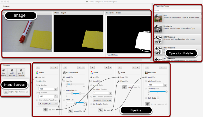
The GRIP user interface consists of 4 parts:
Image Sources are the ways of getting images into the GRIP pipeline. You can provide images through attached cameras or files. Sources are almost always the beginning of the image processing algorithm.
Operation Palette contains the image processing steps from the OpenCV library that you can chain together in the pipeline to form your algorithm. Clicking on an operation in the palette adds it to the end of the pipeline. You can then use the left and right arrows to move the operation within the pipeline.
Pipeline is the sequence of steps that make up the algorithm. Each step (operation) in the pipeline is connected to a previous step from the output of one step to an input to the next step. The data flows from generally from left to right through the connections that you create.
Image Preview are shows previews of the result of each step that has it’s preview button pressed. This makes it easy to debug algorithms by being able to preview the outputs of each intermediate step.
Finding the yellow square
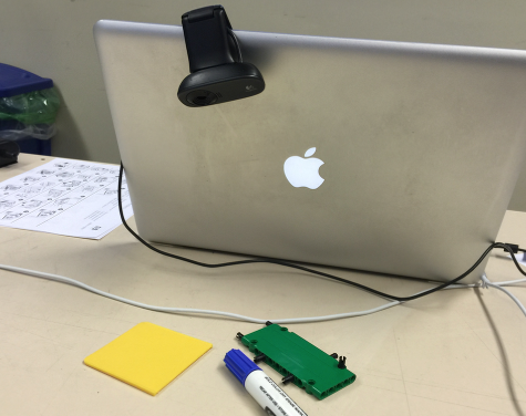
In this application we will try to find the yellow square in the image and display it’s position. The setup is pretty simple, just a USB web camera connected to the computer looking down at some colorful objects. The yellow plastic square is the thing that we’re interested in locating in the image.
Enable the image source
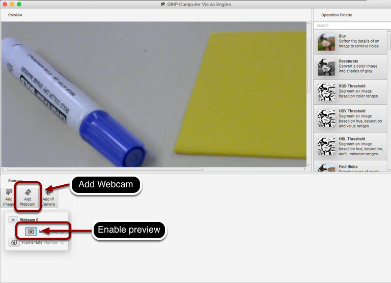
The first step is to acquire an image. To use the source, click on the “Add Webcam” button and select the camera number. In this case the Logitech USB camera that appeared as Webcam 0 and the computer monitor camera was Webcam 1. The web camera is selected in this case to grab the image behind the computer as shown in the setup. Then select the image preview button and the real-time display of the camera stream will be shown in the preview area.
Resize the image
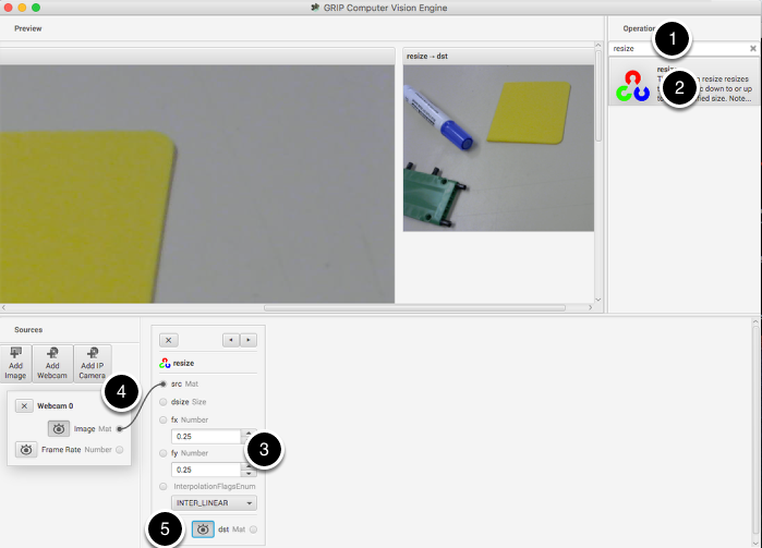
In this case the camera resolution is too high for our purposes, and in fact the entire image cannot even be viewed in the preview window. The “Resize” operation is clicked from the Operation Palette to add it to the end of the pipeline. To help locate the Resize operation, type “Resize” into the search box at the top of the palette. The steps are:
Type “Resize” into the search box on the palette
Click the Resize operation from the palette. It will appear in the pipeline.
Enter the x and y resize scale factor into the resize operation in the pipeline. In this case 0.25 was chosen for both.
Drag from the Webcam image output mat socket to the Resize image source mat socket. A connection will be shown indicating that the camera output is being sent to the resize input.
Click on the destination preview button on the “Resize” operation in the pipeline. The smaller image will be displayed alongside the larger original image. You might need to scroll horizontally to see both as shown.
Lastly, click the Webcam source preview button since there is no reason to look at both the large image and the smaller image at the same time.
Find only the yellow parts of the image
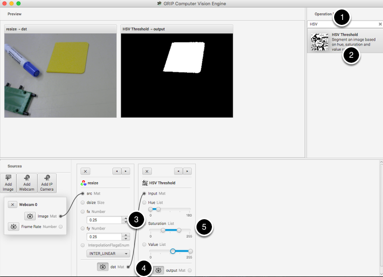
The next step is to remove everything from the image that doesn’t match the yellow color of the piece of plastic that is the object being detected. To do that a HSV Threshold operation is chosen to set upper and lower limits of HSV values to indicate which pixels should be included in the resultant binary image. Notice that the target area is white while everything that wasn’t within the threshold values are shown in black. Again, as before:
Type HSV into the search box to find the HSV Threshold operation.
Click on the operation in the palette and it will appear at the end of the pipeline.
Connect the dst (output) socket on the resize operation to the input of the HSV Threshold.
Enable the preview of the HSV Threshold operation so the result of the operation is displayed in the preview window.
Adjust the Hue, Saturation, and Value parameters only the target object is shown in the preview window.
Get rid of the noise and extraneous hits
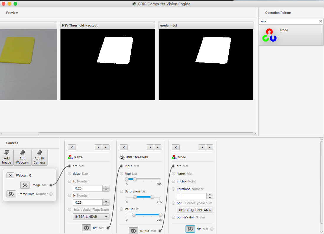
This looks pretty good so far, but sometimes there is noise from other things that couldn’t quite be filtered out. To illustrate one possible technique to reduce those occasional pixels that were detected, an Erosion operation is chosen. Erosion will remove small groups of pixels that are not part of the area of interest.
Mask just the yellow area from the original image
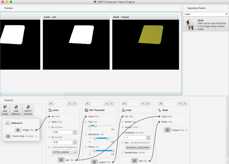
Here a new image is generated by taking the original image and masking (and operation) it with the the results of the erosion. This leaves just the yellow card as seen in the original image with nothing else shown. And it makes it easy to visualize exactly what was being found through the series of filters.
Find the yellow area (blob)
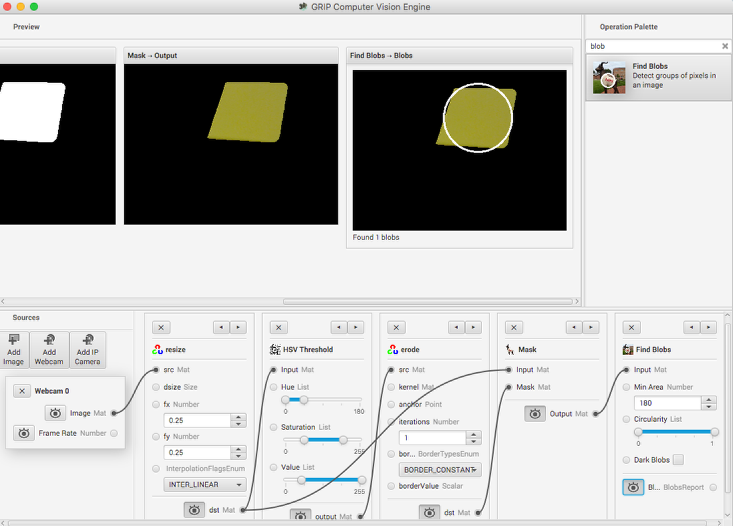
The last step is actually detecting the yellow card using a Blob Detector. This operation looks for a grouping of pixels that have some minimum area. In this case, the only non-black pixels are from the yellow card after the filtering is done. You can see that a circle is drawn around the detected portion of the image. In the release version of GRIP (watch for more updates between now and kickoff) you will be able to send parameters about the detected blob to your robot program using NetworkTables.
Status of GRIP
As you can see from this example, it is very easy and fast to be able to do simple object recognition using GRIP. While this is a very simple example, it illustrates the basic principles of using GRIP and feature extraction in general. Over the coming weeks the project team will be posting updates to GRIP as more features are added. Currently it supports cameras (Axis ethernet camera and web cameras) and image inputs. There is no provision for output yet although NetworkTables and ROS (Robot Operating System) are planned.
You can either download a pre-built release of the code from the GitHub page “Releases” section (https://github.com/WPIRoboticsProjects/GRIP) or you can clone the source repository and built it yourself. Directions on building GRIP are on the project page. There is also additional documentation on the project wiki.
So, please play with GRiP and give us feedback here on the forum. If you find bugs, you can either post them here or as a GitHub project issue on the project page.
Generating Code from GRIP
GRIP Code Generation
When running your vision algorithm on a small processor such as a roboRIO or Raspberry PI it is encouraged to run OpenCV directly on the processor without the overhead of GRIP. To facilitate this, GRIP can generate code in C++, Java, and Python for the pipeline that you have created. This generated code can be added to your robot project and called directly from your existing robot code.
Input sources such as cameras or image directories and output steps such as NetworkTables are not generated. Your code must supply images as OpenCV mats. On the roboRIO, the CameraServer class supplies images in that format. For getting results you can just use generated getter methods for retrieving the resultant values such as contour x and y values.
Generating Code
To generate code, go to Tools > Generate Code. This will bring up a save dialog that lets you create a C++, Java, or Python
class that performs the steps in the GRIP pipeline.

If generating code to be used in a pre-existing project, choose a relevant directory to save the pipeline to.
C++ Users: the pipeline class is split into a header and implementation file
Java Users: the generated class lacks a package declaration, so a declaration should be added to match the directory where the file was saved.
Python Users: the module name will be identical to the class, so the import statement will be something like
from Pipeline import Pipeline
Structure of the Generated Code
Pipeline:
// Process -- this will run the pipeline
process(Mat source)
// Output accessors
getFooOutput()
getBar0Output()
getBar1Output()
...
Running the Pipeline
To run the Pipeline, call the process method with the sources (webcams, IP camera, image file, etc) as arguments. This will
expose the outputs of every operation in the pipeline with the getFooOutput methods.
Getting the Results
Users are able to the outputs of every step in the pipeline. The outputs of these operations would be accessible through their respective accessors. For example:
Operation |
Java/C++ getter |
Python variable |
|---|---|---|
RGB Threshold |
|
|
Blur |
|
|
CV Erode |
|
|
Find Contours |
|
|
Filter Contours |
|
|
If an operation appears multiple times in the pipeline, the accessors for those operations have the number of that operation:
Operation |
Which appearance |
Accessor |
|---|---|---|
Blur |
First |
|
Blur |
Second |
|
Blur |
Third |
|
Using Generated Code in a Robot Program
GRIP generates a class that can be added to an FRC® program that runs on a roboRIO and without a lot of additional code, drive the robot based on the output.
Included here is a complete sample program that uses a GRIP pipeline that drives a robot towards a piece of retroreflective material.
This program is designed to illustrate how the vision code works and does not necessarily represent the best technique for writing your robot program. When writing your own program be aware of the following considerations:
Using the camera output for steering the robot could be problematic. The camera code in this example that captures and processes images runs at a much slower rate that is desirable for a control loop for steering the robot. A better, and only slightly more complex solution, is to get headings from the camera and it’s processing rate, then have a much faster control loop steering to those headings using a gyro sensor.
Keep the vision code in the class that wraps the pipeline. A better way of writing object oriented code is to subclass or instantiate the generated pipeline class and process the OpenCV results there rather than in the robot program. In this example, the robot code extracts the direction to drive by manipulating the resultant OpenCV contours. By having the OpenCV code exposed throughout the robot program it makes it difficult to change the vision algorithm should you have a better one.
Iterative program definitions
package org.usfirst.frc.team190.robot;
import org.usfirst.frc.team190.grip.MyVisionPipeline;
import org.opencv.core.Rect;
import org.opencv.imgproc.Imgproc;
import edu.wpi.cscore.UsbCamera;
import edu.wpi.first.cameraserver.CameraServer;
import edu.wpi.first.wpilibj.drive.DifferentialDrive;
import edu.wpi.first.wpilibj.PWMSparkMax;
import edu.wpi.first.wpilibj.TimedRobot;
import edu.wpi.first.vision.VisionRunner;
import edu.wpi.first.vision.VisionThread;
public class Robot extends TimedRobot {
private static final int IMG_WIDTH = 320;
private static final int IMG_HEIGHT = 240;
private VisionThread visionThread;
private double centerX = 0.0;
private DifferentialDrive drive;
private PWMSparkMax left;
private PWMSparkMax right;
private final Object imgLock = new Object();
In this first part of the program you can see all the import statements for the WPILib classes used for this program.
The image width and height are defined as 320x240 pixels.
The VisionThread is a WPILib class makes it easy to do your camera processing in a separate thread from the rest of the robot program.
centerX value will be the computed center X value of the detected target.
DifferentialDrive encapsulates the drive motors on this robot and allows simplified driving.
imgLock is a variable to synchronize access to the data being simultaneously updated with each image acquisition pass and the code that’s processing the coordinates and steering the robot.
@Override
public void robotInit() {
UsbCamera camera = CameraServer.startAutomaticCapture();
camera.setResolution(IMG_WIDTH, IMG_HEIGHT);
visionThread = new VisionThread(camera, new MyVisionPipeline(), pipeline -> {
if (!pipeline.filterContoursOutput().isEmpty()) {
Rect r = Imgproc.boundingRect(pipeline.filterContoursOutput().get(0));
synchronized (imgLock) {
centerX = r.x + (r.width / 2);
}
}
});
visionThread.start();
left = new PWMSparkMax(0);
right = new PWMSparkMax(1);
drive = new DifferentialDrive(left, right);
}
The robotInit() method is called once when the program starts up. It creates a CameraServer instance that begins capturing images at the requested resolution (IMG_WIDTH by IMG_HEIGHT).
Next an instance of the class VisionThread is created. VisionThread begins capturing images from the camera asynchronously in a separate thread. After processing each image, the pipeline computed bounding box around the target is retrieved and it’s center X value is computed. This centerX value will be the x pixel value of the center of the rectangle in the image.
The VisionThread also takes a VisionPipeline instance (here, we have a subclass MyVisionPipeline generated by GRIP) as well as a callback that we use to handle the output of the pipeline. In this example, the pipeline outputs a list of contours (outlines of areas in an image) that mark goals or targets of some kind. The callback finds the bounding box of the first contour in order to find its center, then saves that value in the variable centerX. Note the synchronized block around the assignment: this makes sure the main robot thread will always have the most up-to-date value of the variable, as long as it also uses synchronized blocks to read the variable.
@Override
public void autonomousPeriodic() {
double centerX;
synchronized (imgLock) {
centerX = this.centerX;
}
double turn = centerX - (IMG_WIDTH / 2);
drive.arcadeDrive(-0.6, turn * 0.005);
}
This, the final part of the program, is called repeatedly during the autonomous period of the match. It gets the centerX pixel value of the target and subtracts half the image width to change it to a value that is zero when the rectangle is centered in the image and positive or negative when the target center is on the left or right side of the frame. That value is used to steer the robot towards the target.
Note the synchronized block at the beginning. This takes a snapshot of the most recent centerX value found by the VisionThread.
Using GRIP with a Kangaroo Computer
A recently available computer called the Kangaroo looks like a great platform for running GRIP on FRC® robots. Some of the specs for this processor include:
Quad core 1.4Ghz Atom processor
HDMI port
2 USB ports (1 USB2 and 1 USB3)
2GB RAM
32GB Flash
Flash card slot
WiFi
Battery with 4 hours running time
Power supply
Windows 10
and a fingerprint reader
The advantage of this setup is that it offloads the roboRIO from doing image processing and it is a normal Windows system so all of our software should work without modification. Be sure to read the caveats at the end of this page before jumping in.
More detailed instructions for using a Kangaroo for running GRIP can be found in the following PDF document created by Scott Taylor and FRC 1735. His explanation goes beyond what is shown here, detailing how to get the GRIP program to auto-start on boot and many other details.
Setup
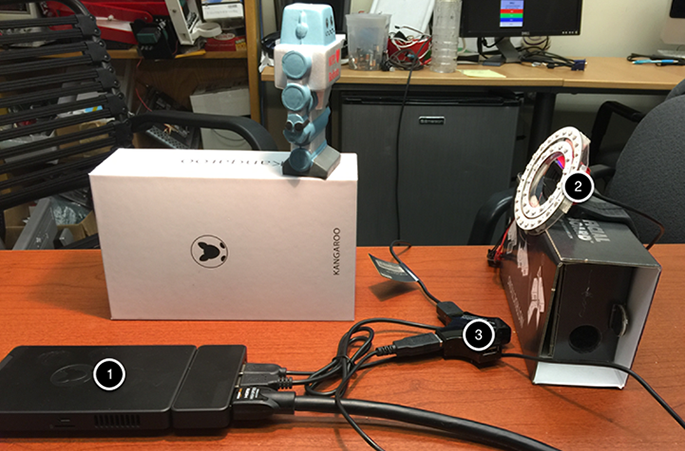
The nice thing about this setup is that you just need to plug in a monitor, keyboard, mouse and (in this case) the Microsoft web camera and you are good to go with programming the GRIP pipeline. When you are finished, disconnect the keyboard, mouse and monitor and put the Kangaroo on your robot. You will need to disable the WiFi on the Kangaroo and connect it to the robot with a USB ethernet dongle to the extra ethernet port on the robot radio.
In this example you can see the Kangaroo computer (1) connected to a USB hub (3), keyboard, and an HDMI monitor for programming. The USB hub is connected to the camera and mouse.
Sample GRIP program
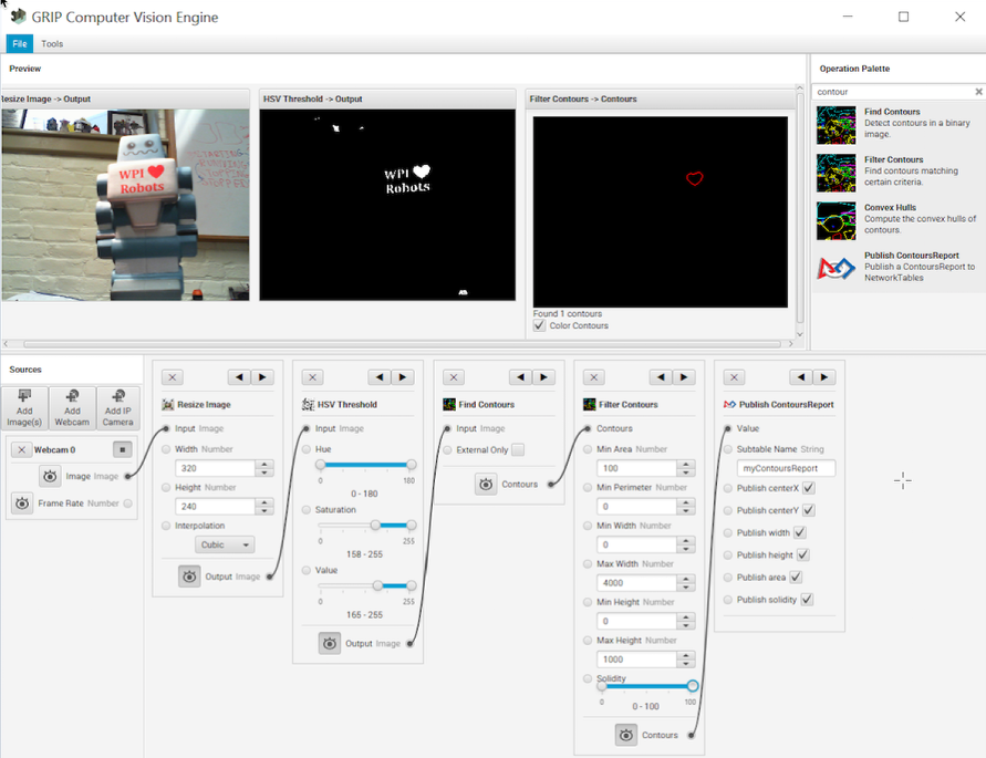
Attached is the sample program running on the Kangaroo detecting the red heart on the little foam robot in the image (left panel). It is doing a HSV threshold to only get that red color then finding contours, and then filtering the contours using the size and solidity. At the end of the pipeline, the values are being published to NetworkTables.
Viewing Contours Report in NetworkTables
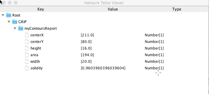
This is the output from the OutlineViewer (<username>/WPILib/tools/OutlineViewer.jar), running on a different computer as a server (since there is no roboRIO on the network in this example) and the values being reported back for the single contour that the program detected that met the requirements of the Filter Contours operation.
Considerations
The Kangaroo runs Windows 10, so care must to be taken to make sure GRIP will keep running on the robot during a match or testing. For example, it should not try to do a Windows Update, Virus scan refresh, go to sleep, etc. Once configured, it has the advantage of being a normal Intel Architecture and should give predictable performance since it is running only one application.
Vision on the RoboRIO
Using the CameraServer on the roboRIO
Simple CameraServer Program
The following program starts automatic capture of a USB camera like the Microsoft LifeCam that is connected to the roboRIO. In this mode, the camera will capture frames and send them to the dashboard. To view the images, create a CameraServer Stream Viewer widget using the “View”, then “Add” menu in the dashboard. The images are unprocessed and just forwarded from the camera to the dashboard.
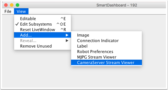
package org.usfirst.frc.team190.robot;
import edu.wpi.first.cameraserver.CameraServer;
import edu.wpi.first.wpilibj.IterativeRobot;
public class Robot extends IterativeRobot {
public void robotInit() {
CameraServer.startAutomaticCapture();
}
}
#include "cameraserver/CameraServer.h"
class Robot: public IterativeRobot
{
private:
void RobotInit()
{
frc::CameraServer::StartAutomaticCapture();
}
};
START_ROBOT_CLASS(Robot)
Advanced Camera Server Program
In the following example a thread created in robotInit() gets the Camera Server instance. Each frame of the video is individually processed, in this case converting a color image (BGR) to gray scale using the OpenCV cvtColor() method. The resultant images are then passed to the output stream and sent to the dashboard. You can replace the cvtColor operation with any image processing code that is necessary for your application. You can even annotate the image using OpenCV methods to write targeting information onto the image being sent to the dashboard.
package org.usfirst.frc.team190.robot;
import org.opencv.core.Mat;
import org.opencv.imgproc.Imgproc;
import edu.wpi.cscore.CvSink;
import edu.wpi.cscore.CvSource;
import edu.wpi.cscore.UsbCamera;
import edu.wpi.first.cameraserver.CameraServer;
import edu.wpi.first.wpilibj.IterativeRobot;
public class Robot extends IterativeRobot {
public void robotInit() {
new Thread(() -> {
UsbCamera camera = CameraServer.startAutomaticCapture();
camera.setResolution(640, 480);
CvSink cvSink = CameraServer.getVideo();
CvSource outputStream = CameraServer.putVideo("Blur", 640, 480);
Mat source = new Mat();
Mat output = new Mat();
while(!Thread.interrupted()) {
if (cvSink.grabFrame(source) == 0) {
continue;
}
Imgproc.cvtColor(source, output, Imgproc.COLOR_BGR2GRAY);
outputStream.putFrame(output);
}
}).start();
}
}
#include "cameraserver/CameraServer.h"
#include <opencv2/imgproc/imgproc.hpp>
#include <opencv2/core/core.hpp>
class Robot: public IterativeRobot
{
private:
static void VisionThread()
{
cs::UsbCamera camera = frc::CameraServer::StartAutomaticCapture();
camera.SetResolution(640, 480);
cs::CvSink cvSink = frc::CameraServer::GetVideo();
cs::CvSource outputStreamStd = frc::CameraServer::PutVideo("Gray", 640, 480);
cv::Mat source;
cv::Mat output;
while(true) {
if (cvSink.GrabFrame(source) == 0) {
continue;
}
cvtColor(source, output, cv::COLOR_BGR2GRAY);
outputStreamStd.PutFrame(output);
}
}
void RobotInit()
{
std::thread visionThread(VisionThread);
visionThread.detach();
}
};
START_ROBOT_CLASS(Robot)
Notice that in these examples, the PutVideo() method writes the video to a named stream. To view that stream on Shuffleboard, select that named stream. In this case that is “Blur” for the Java program and “Gray” for the C++ sample.
Using Multiple Cameras
Switching the Driver Views
If you’re interested in just switching what the driver sees, and are using SmartDashboard, the SmartDashboard CameraServer Stream Viewer has an option (“Selected Camera Path”) that reads the given NetworkTables key and changes the “Camera Choice” to that value (displaying that camera). The robot code then just needs to set the NetworkTables key to the correct camera name. Assuming “Selected Camera Path” is set to “CameraSelection”, the following code uses the joystick 1 trigger button state to show camera1 and camera2.
UsbCamera camera1;
UsbCamera camera2;
Joystick joy1 = new Joystick(0);
NetworkTableEntry cameraSelection;
@Override
public void robotInit() {
camera1 = CameraServer.startAutomaticCapture(0);
camera2 = CameraServer.startAutomaticCapture(1);
cameraSelection = NetworkTableInstance.getDefault().getTable("").getEntry("CameraSelection");
}
@Override
public void teleopPeriodic() {
if (joy1.getTriggerPressed()) {
System.out.println("Setting camera 2");
cameraSelection.setString(camera2.getName());
} else if (joy1.getTriggerReleased()) {
System.out.println("Setting camera 1");
cameraSelection.setString(camera1.getName());
}
}
cs::UsbCamera camera1;
cs::UsbCamera camera2;
frc::Joystick joy1{0};
nt::NetworkTableEntry cameraSelection;
void RobotInit() override {
camera1 = frc::CameraServer::StartAutomaticCapture(0);
camera2 = frc::CameraServer::StartAutomaticCapture(1);
cameraSelection = nt::NetworkTableInstance::GetDefault().GetTable("")->GetEntry("CameraSelection");
}
void TeleopPeriodic() override {
if (joy1.GetTriggerPressed()) {
std::cout << "Setting Camera 2" << std::endl;
cameraSelection.SetString(camera2.GetName());
} else if (joy1.GetTriggerReleased()) {
std::cout << "Setting Camera 1" << std::endl;
cameraSelection.SetString(camera1.GetName());
}
}
If you’re using some other dashboard, you can change the camera used by the camera server dynamically. If you open a stream viewer nominally to camera1, the robot code will change the stream contents to either camera1 or camera2 based on the joystick trigger.
UsbCamera camera1;
UsbCamera camera2;
VideoSink server;
Joystick joy1 = new Joystick(0);
@Override
public void robotInit() {
camera1 = CameraServer.startAutomaticCapture(0);
camera2 = CameraServer.startAutomaticCapture(1);
server = CameraServer.getServer();
}
@Override
public void teleopPeriodic() {
if (joy1.getTriggerPressed()) {
System.out.println("Setting camera 2");
server.setSource(camera2);
} else if (joy1.getTriggerReleased()) {
System.out.println("Setting camera 1");
server.setSource(camera1);
}
}
cs::UsbCamera camera1;
cs::UsbCamera camera2;
cs::VideoSink server;
frc::Joystick joy1{0};
bool prevTrigger = false;
void RobotInit() override {
camera1 = frc::CameraServer::StartAutomaticCapture(0);
camera2 = frc::CameraServer::StartAutomaticCapture(1);
server = frc::CameraServer::GetServer();
}
void TeleopPeriodic() override {
if (joy1.GetTrigger() && !prevTrigger) {
std::cout << "Setting Camera 2" << std::endl;
server.SetSource(camera2);
} else if (!joy1.GetTrigger() && prevTrigger) {
std::cout << "Setting Camera 1" << std::endl;
server.SetSource(camera1);
}
prevTrigger = joy1.GetTrigger();
}
Keeping Streams Open
By default, the cscore library is pretty aggressive in turning off cameras not in use. What this means is that when you switch cameras, it may disconnect from the camera not in use, so switching back will have some delay as it reconnects to the camera. To keep both camera connections open, use the SetConnectionStrategy() method to tell the library to keep the streams open, even if you aren’t using them.
UsbCamera camera1;
UsbCamera camera2;
VideoSink server;
Joystick joy1 = new Joystick(0);
@Override
public void robotInit() {
camera1 = CameraServer.startAutomaticCapture(0);
camera2 = CameraServer.startAutomaticCapture(1);
server = CameraServer.getServer();
camera1.setConnectionStrategy(ConnectionStrategy.kKeepOpen);
camera2.setConnectionStrategy(ConnectionStrategy.kKeepOpen);
}
@Override
public void teleopPeriodic() {
if (joy1.getTriggerPressed()) {
System.out.println("Setting camera 2");
server.setSource(camera2);
} else if (joy1.getTriggerReleased()) {
System.out.println("Setting camera 1");
server.setSource(camera1);
}
}
cs::UsbCamera camera1;
cs::UsbCamera camera2;
cs::VideoSink server;
frc::Joystick joy1{0};
bool prevTrigger = false;
void RobotInit() override {
camera1 = frc::CameraServer::StartAutomaticCapture(0);
camera2 = frc::CameraServer::StartAutomaticCapture(1);
server = frc::CameraServer::GetServer();
camera1.SetConnectionStrategy(cs::VideoSource::ConnectionStrategy::kConnectionKeepOpen);
camera2.SetConnectionStrategy(cs::VideoSource::ConnectionStrategy::kConnectionKeepOpen);
}
void TeleopPeriodic() override {
if (joy1.GetTrigger() && !prevTrigger) {
std::cout << "Setting Camera 2" << std::endl;
server.SetSource(camera2);
} else if (!joy1.GetTrigger() && prevTrigger) {
std::cout << "Setting Camera 1" << std::endl;
server.SetSource(camera1);
}
prevTrigger = joy1.GetTrigger();
}
Note
If both cameras are USB, you may run into USB bandwidth limitations with higher resolutions, as in all of these cases the roboRIO is going to be streaming data from both cameras to the roboRIO simultaneously (for a short period in options 1 and 2, and continuously in option 3). It is theoretically possible for the library to avoid this simultaneity in the option 2 case (only), but this is not currently implemented.
Different cameras report bandwidth usage differently. The library will tell you if you’re hitting the limit; you’ll get this error message:
could not start streaming due to USB bandwidth limitations;
try a lower resolution or a different pixel format
(VIDIOC_STREAMON: No space left on device)
If you’re using Option 3 it will give you this error during RobotInit(). Thus you should just try your desired resolution and adjusting as necessary until you both don’t get that error and don’t exceed the radio bandwidth limitations.
Vision with an Axis Camera
Configuring an Axis Camera
Note
Three different Axis camera models are supported by the FRC® software, the Axis 206, Axis M1011 and Axis M1013. This document provides instructions on how to configure one of these cameras for FRC use. To follow the instructions in this document, you must have installed the NI FRC Game Tools and Configured your radio
Connect the camera
Connect the Axis camera to the radio using an Ethernet cable. Connect your computer to the radio using an Ethernet cable or via a wireless connection.
Axis Camera Setup Tool
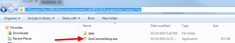
Browse to C:\Program Files (x86)\National Instruments\LabVIEW 2019\project\Axis Camera Tool and double-click on AxisCameraSetup.exe to start the Axis Camera Setup Tool.
Tool Overview
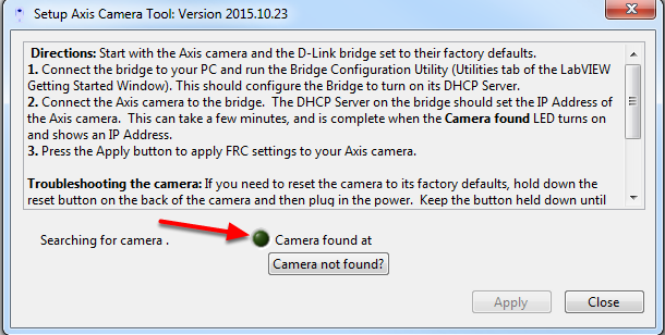
The camera should be automatically detected and the green indicator light should be lit. If it is not, make sure the camera is powered on (the ring on the camera face should be green) and connected to your computer. If the indicator remains off follow the instructions in the tool textbox next to Troubleshooting the camera to reset the camera. You can also use the “Camera not found?” button to check the IP address of your computer, one of the addresses listed should be of the form 10.TE.AM.XX where TEAM is your 4 digit team number.
Setup the Camera
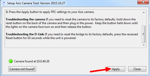
To configure the camera, press Apply. This will configure many of the necessary/recommended settings for using the camera for FRC. Currently the tool does not properly configure the DNS name of the camera in many cases.
Camera Webpage
To set the network settings, open a web browser and enter the address shown next to Camera found at in the tool (in the example above this is 10.0.40.20) in the address bar and press enter. You should see a Configure Root Password page, set this password to whatever you would like, but admin is recommended.
Configure Basic Network Settings
To configure the network settings of the camera, click the arrow to expand the System Options pane, then click the arrow to expand Network, then expand TCP/IP and select Basic. Set the camera to obtain an IP address via DHCP by selecting the bubble. Alternately, you may choose to set a static IP in the range 10.TE.AM.3 to 10.TE.AM.19. This is outside the range handed out by the radio (home use) or FMS system (event use) so you will avoid any IP conflicts.
Click Save.
Configure Advanced Network Settings
Next click Advanced under TCP/IP. Set the Host Name Configuration to “Use the host name:” and set the value to axis-camera as shown. If you plan to use multiple cameras on your robot, select a unique host name for each. You will need to modify the dashboard and/or robot code to work with the additional cameras and unique host names.
Click Save.
Manual Camera Configuration
It is recommended to use the Setup Axis Camera Tool to configure the Axis Camera. If you need to configure the camera manually, connect the camera directly to the computer, configure your computer to have a static IP of 192.168.0.5, then open a web browser and enter 192.168.0.90 in the address bar and press enter. You should see a Configure Root Password page, set this password to whatever you would like, but admin is recommended.
If you do not see the camera webpage come up, you may need to reset the camera to factory defaults. To do this, remove power from the camera, hold the reset button while applying power to the camera and continue holding it until the lights on the camera face turn on, then release the reset button and wait for the lights to turn green. The camera is now reset to factory settings and should be accessible via the 192.168.0.90 address.
Click Setup to go to the setup page.
Manual - Configure Users
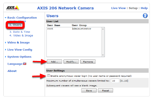
On the left side click Users to open the users page. Click Add then enter the Username FRC Password FRC and click the Administrator bubble, then click OK. If using the SmartDashboard, check the Enable anonymous viewer login box. Then click Save.
Manual - Configure Image Settings
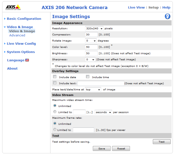
Click Video & Image on the left side to open the image settings page. Set the Resolution and Compression to the desired values (recommended 320x240, 30). To limit the framerate to under 30 FPS, select the Limited to bubble under Maximum frame rate and enter the desired rate in the box. Color, Brightness and Sharpness may also be set on this screen if desired. Click Save when finished.
Manual - Configure Basic Network Settings
To configure the network settings of the camera, click the arrow to expand the System Options pane, then click the arrow to expand Network, then expand TCP/IP and select Basic. Set the camera to obtain an IP address via DHCP by selecting the bubble. Alternately, you may choose to set a static IP in the range 10.TE.AM.3 to 10.TE.AM.19. This is outside the range handed out by the radio (home use) or FMS system (event use) so you will avoid any IP conflicts.
Click Save.
Manual - Configure Advanced Network Settings
Next click Advanced under TCP/IP. Set the Host Name Configuration to “Use the host name:” and set the value to axis-camera as shown. If you plan to use multiple cameras on your robot, select a unique host name for each. You will need to modify the dashboard and/or robot code to work with the additional cameras and unique host names.
Click Save.
Axis M1013 Camera Compatibility
The Axis M1011 camera has been discontinued and superseded by the Axis M1013 camera. This document details the differences between the two cameras when used with WPILib and the provided sample vision programs.
Optical Differences
The Axis M1013 camera has a few major optical differences from the M1011 camera:
The M1013 is an adjustable focus camera. Make sure to focus your M1013 camera by turning the grey and black lens housing to make sure you have a clear image at your desired viewing distance.
The M1013 has a wider view angle (67°) compared to the M1011 (47°). This means that for a feature of a fixed size, the image of that feature will span a smaller number of pixels
Using the M1013 with WPILib
The M1013 camera has been tested with all of the available WPILib parameters and the following performance exceptions were noted:
The M1013 does not support the 160x120 resolution. Requesting a stream of this resolution will result in no images being returned or displayed.
The M1013 does not appear to work with the Color Enable parameter exposed by WPILib. Regardless of the setting of this parameter a full color image was returned.
All other WPILib camera parameters worked as expected. If any issues not noted here are discovered, please file a bug report on GitHub.
Camera Settings
It is very difficult to achieve good image processing results without good images. With a light mounted near the camera lens, you should be able to use the provided examples, the LabVIEW Dashboard or Shuffleboard, NI Vision Assistant or a web browser to view camera images and experiment with camera settings.
Changing Camera Settings
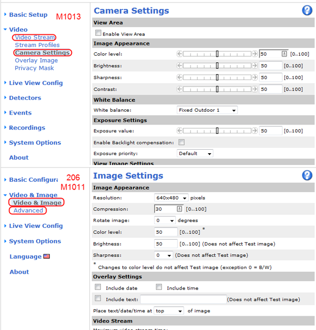
To change the camera settings on any of the supported Axis cameras (206, M1011, M1013), browse to the camera’s webpage by entering its address (usually 10.TE.AM.11) in a web browser. Click Setup near the top right corner of the page. On the M1013, the settings listed below are split between the Video Stream page and the Camera Settings page, both listed under the Video section.
Focus
The Axis M1011 has a fixed-focus lens and no adjustment is needed. The Axis 206 camera has a black bezel around the lens that rotates to move the lens in and out and adjust focus. The Axis M1013 has a silver and black bezel assembly around the lens to adjust the focus. Ensure that the images you are processing are relatively sharp and focused for the distances needed on your robot.
Compression
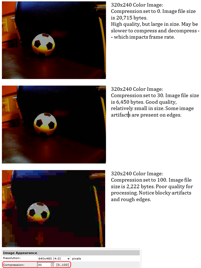
The Axis camera returns images in BMP, JPEG, or MJPEG format. BMP images are quite large and take more time to transmit to the roboRIO and laptop. Therefore the WPILib implementations typically use MJPEG (motion JPEG). The compression setting ranges from 0 to 100, with 0 being very high quality images with very little compression, and 100 being very low quality images with very high compression. The camera default is 30, and it is a good compromise, with few artifacts that will degrade image processing.
Note
Teams are advised to consider how the compression setting on the camera affects bandwidth if performing processing on the Driver Station computer, see the FMS Whitepaper for more details.
Resolution
Image sizes shared by the supported cameras are 160x120, 320x240, and 640x480. The M1011 and 1013 have additional sizes, but they aren’t built into WPILib. The largest image size has four times as many pixels that are one-fourth the size of the middle size image. The large image has sixteen times as many pixels as the small image.
The tape used on the target is 4 inches (~10 cm) wide, and for good processing, you will want that 4 inch (~10 cm) feature to be at least two pixels wide. Using the distance equations above, we can see that a medium size image should be fine up to the point where the field of view is around 640 inches (~16 m), a little over 53 feet (~16 m), which is nearly double the width of the FRC® field. This occurs at around 60 feet (~18 m) away, longer than the length of the field. The small image size should be usable for processing to a distance of about 30 feet (~9 m) or a little over mid-field.
Image size also impacts the time to decode and to process. Smaller images will be roughly four times faster than the next size up. If the robot or target is moving, it is quite important to minimize image processing time since this will add to the delay between the target location and perceived location. If both robot and target are stationary, processing time is typically less important.
Note
When requesting images using LabVIEW (either the Dashboard or Robot Code), the resolution and Frame Rate settings of the camera will be ignored. The LabVIEW code specifies the framerate and resolution as part of the stream request (this does not change the settings stored in the camera, it overrides that setting for the specific stream). The SmartDashboard and robot code in C++ or Java will use the resolution and framerate stored in the camera.
Frame Rate
The Axis Cameras have a max framerate of 30 frames per second. If desired, a limit can be set lower to reduce bandwidth consumption.
Color Enable
The Axis cameras typically return color images, but are capable of disabling color and returning a monochrome or grayscale image. The resulting image is a bit smaller in file size, and considerably quicker to decode. If processing is carried out only on the brightness or luminance of the image, and the color of the ring light is not used, this may be a useful technique for increasing the frame rate or lowering the CPU usage.
White Balance
If the color of the light shine is being used to identify the marker, be sure to control the camera settings that affect the image coloring. The most important setting is white balance. It controls how the camera blends the component colors of the sensor in order to produce an image that matches the color processing of the human brain. The camera has five or six named presets, an auto setting that constantly adapts to the environment, and a hold setting – for custom calibration.
The easiest approach is to use a named preset, one that maintains the saturation of the target and doesn’t introduce problems by tinting neutral objects with the color of the light source.
To custom-calibrate the white balance, place a known neutral object in front of the camera. A sheet of white paper is a reasonable object to start with. Set the white balance setting to auto, wait for the camera to update its filters (ten seconds or so), and switch the white balance to hold.
Exposure
The brightness or exposure of the image also has an impact on the colors being reported. The issue is that as overall brightness increases, color saturation will start to drop. Lets look at an example to see how this occurs. A saturated red object placed in front of the camera will return an RGB measurement high in red and low in the other two e.g. (220, 20, 30). As overall white lighting increases, the RGB value increases to (240, 40, 50), then (255, 80, 90), then (255, 120, 130), and then (255, 160, 170). Once the red component is maximized, additional light can only increase the blue and green, and acts to dilute the measured color and lower the saturation. If the point is to identify the red object, it is useful to adjust the exposure to avoid diluting your principal color. The desired image will look somewhat dark except for the colored shine.
There are two approaches to control camera exposure times. One is to allow the camera to compute the exposure settings automatically, based on its sensors, and then adjust the camera’s brightness setting to a small number to lower the exposure time. The brightness setting acts similar to the exposure compensation setting on SLR cameras. The other approach is to calibrate the camera to use a custom exposure setting. To do this on a 206 or M1011, change the exposure setting to auto, expose the camera to bright lights so that it computes a short exposure, and then change the exposure setting to hold. Both approaches will result in an overall dark image with bright saturated target colors that stand out from the background and are easier to mask.
The M1013 exposure settings look a little different. The Enable Backlight compensation option is similar to the Auto exposure settings of the M1011 and 206 and you will usually want to un-check this box. Adjust the Brightness and Exposure value sliders until your image looks as desired. The Exposure Priority should generally be set to Motion. This will prioritize framerate over image quality. Note that even with these settings the M1013 camera still performs some auto exposure compensation so it is recommended to check calibration frequently to minimize any impact lighting changes may have on image processing. See Calibration for more details.
Calibration
While many of the numbers for the Vision Processing code can be determined theoretically, there are a few parameters that are typically best to measure empirically then enter back into the code (a process typically known as calibration). This article will show how to perform calibration for the Color (masking), and View Angle (distance) using the NI Vision Assistant. If you are using C++ or Java and have not yet installed the NI Vision Assistant, see the article Installing NI Vision Assistant.
Enable Snapshots
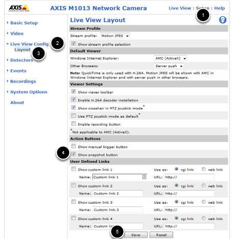
To capture snapshots from the Axis camera, you must first enable the Snapshot button. Open a web-browser and browse to camera’s address (10.TE.AM.11), enter the Username/Password combo FRC/FRC if prompted, then click Setup->Live View Config->Layout. Click on the checkbox to Show snapshot button then click Save.
Check Camera Settings
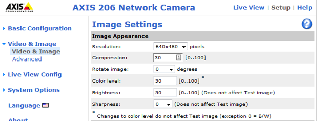
Depending on how you are capturing the image stream in your program, it may be possible to stream a different resolution, framerate and/or compression than what is saved in the camera and used in the Live View. Before performing any calibration it is recommended you verify that the settings in the camera match the settings in your code. To check the settings in the camera, click on the Video and Image header on the left side of the screen, then click Video and Image.
Capture Images
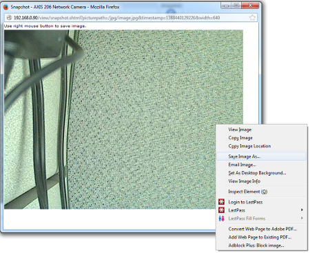
Click the Live View button to return to the Live View page and you should now see a Snapshot button. Clicking this button opens a pop-up window with a static image capture. Right-click on this image, select Save Image as and select your desired location and file name, then save the image.
Load Image(s) in Vision Assistant
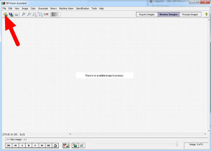
Open the NI Vision Assistant and select the Browse Images option. Select the Open Images icon in the top left of the Toolbar, then locate your images. Repeat as necessary to load all desired images.
Color Threshold
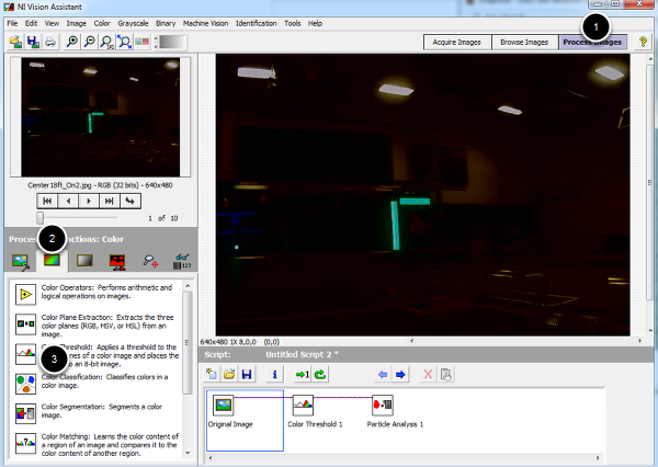
Click Process Images in the top right, then select the color tab on the bottom right and click the Color Threshold icon.
HSV Calibration
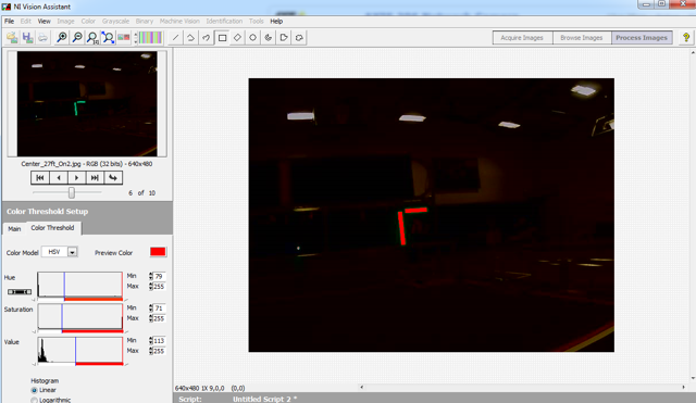
Change the Color Model dropdown to HSV. Next tune the window on each of the three values to cover as much of the target as possible while filtering everything else. If using a green light, you may want to use the values in the sample code as a starting point. If you have multiple images you can use the controls in the top left to cycle through them. Use the center two arrow controls or the slider to change the preview image in the top left window, then click the right-most arrow to make it the active image. When you are happy with the values you have selected, note down the ranges for the Hue, Saturation and Value. You will need to enter these into the appropriate place in the vision code. Click OK to finish adding the step to the script.
You may wish to take some new sample images using the time for camera calibration at your event to verify or tweak your ranges slightly based on the venue lighting conditions.
View Angle/Distance Calibration
While a theoretical view angle for each camera model can be found in the datasheet, empirical testing has found that these numbers may be a bit off even for the horizontal view angle. Given that this year’s code uses the vertical field-of-view it is best to perform your own calibration for your camera (though empirical values for each camera type are included in the code as a reference). To do this set up an equation where the view angle, θ, is the only unknown. To do this, utilize a target of known size at a known distance, leaving the view angle as the only unknown. Let’s take our equation from the previous article, \(d = T_{\mathrm{ft}} \cdot \frac{\textit{FOV}_{\mathrm{pixel}}}{T_{\mathrm{pixel}}\tan\theta}\), and re-arrange it to solve for θ:
Taking Measurements
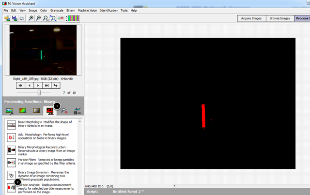
One way to take the required measurements is to use the same images of the retro-reflective tape that were used for the color calibration above. We can use Vision Assistant to provide the height of the detected blob in pixels. By measuring the real-world distance between the camera and the target, we now have all of the variables to solve our equation for the view angle.
To measure the particles in the image, click the Binary tab, then click the Particle Analysis icon.
Selecting Measurements
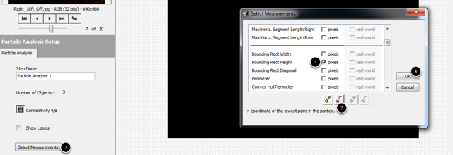
Click on the Select Measurements button. In this case, we are only interested in the bounding box height. Click on the button with the X to deselect all measurements, then locate the Bounding Rect Height measurement and check the box. Click OK to save.
Measuring the Particle
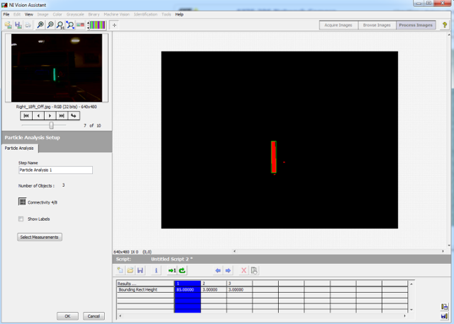
The measurements for each particle will now be displayed in the window at the bottom of the screen. If your image has multiple particles, you can click in each box to have Vision Assistant highlight the particle so you can make sure you have the right one. This article will show the calculation using a single image, but you may wish to perform the calculation on multiple images from multiple distances and use a technique such as averaging or least squares fit to determine the appropriate value for the View angle. You can use the same arrow controls described in the color section above to change the active image.
Calculation
As seen in the previous step, the particle representing the 32in tall vertical target in this example measured 85 pixels tall in a 640x480 image. The image shown was taken from (very roughly) 18 ft. away. Plugging these numbers into the equation from above….
Depending on what you use to calculate the arctangent, your answer may be in radians, make sure to convert back to degrees if entering directly into the sample code as the view angle.
Note
The code uses View Angle and we just calculated θ. Make sure to multiply θ by 2 if replacing the constants in the code. Multiplying our result by 2 yields 45.3°. This image is from a M1013 camera, so our value is a bit off from the previously measured 29.1 but given that the 18ft. was a very rough measurement this shows that we are in the ballpark and likely performed the calculation correctly.
Using the Axis Camera at Single Network Events
The convention for using the Axis camera uses mDNS with the camera name set to axis-camera.local. At home, this works fine as there is only one camera on the network. At official events, this works fine as each team is on their own VLAN and therefore doesn’t have visibility to another team’s camera. However, at an off-season event using a single network, this will cause an issue where all teams will connect to whichever team’s camera “wins” the mDNS resolution and becomes axis-camera. The other cameras will see that the name is taken and use an alternative name. This article describes how to modify the Dashboard and/or robot code to use a different mDNS name to separate the camera streams.
Changing the Camera mDNS Name
To change the mDNS name in the camera, follow the instructions in Configuring an Axis Camera, but substitute the new name such as axis-cameraTEAM where TEAM is your team number.
Viewing the Camera on the DS PC - Browser or SmartDashboard
If you are using a web-browser or SmartDashboard (which accepts mDNS names for the Simple Camera Viewer widget), updating to use the new mDNS name is simple. Simply change the URL in the browser or the address in the Simple Camera Viewer widget properties to the new mDNS name and you are all set.
Viewing the Camera on the DS PC - LabVIEW Dashboard
To view the camera stream in the LabVIEW Dashboard, you will need to build a customized version of the Dashboard. Note that this customized version will only work for the Axis camera and will no longer work for a USB camera. Revert to the default Dashboard to use a USB camera.
Creating a Dashboard Project
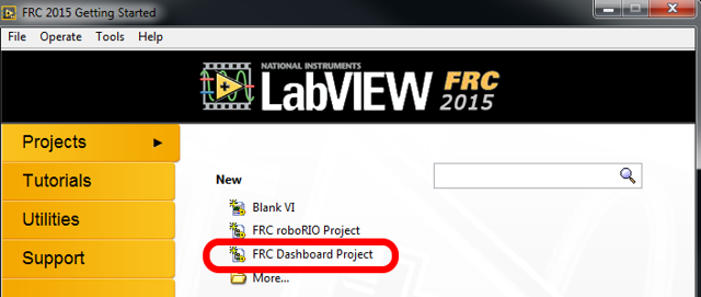
From the LabVIEW Splash screen, select “FRC® Dashboard Project”. Name the project as desired, then click Finish.
Locating Loop 2 - Camera IP
Double click on Dashboard Main.vi in the project explorer to open it and press Ctrl+E to see the block diagram. Scroll down to the loop with the comment that says Loop 2 and locate the “Camera IP” input.
Editing the Camera IP
Delete the Camera IP node, right click on the broken wire and click Create Constant (connect the constant to the wire if necessary). In the box, enter the mDNS name of your camera with a .local suffix (e.g. axis-cameraTEAM.local where TEAM is replaced with your team number). The example above shows a sample name for team 9999. Then click File->Save or Ctrl+S to save the VI.
Note
You may also wish to make a minor modification to the Front Panel to verify that you are running the right dashboard later.
Building the Dashboard
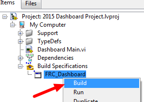
To build the new dashboard, expand Build Specifications in the Project Explorer, right click on FRC_Dashboard and select Build.
Setting the Driver Station to Launch the Modified Dashboard
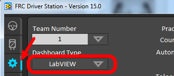
On the Setup tab of the Driver Station, change to dropdown box to LabVIEW to launch your new Dashboard.
Accessing the Camera from Robot Code
If you wish to access the renamed camera from your robot code, you will have to modify it as well. In C++ and Java, just change the String used for the camera host name to match the new name. In LabVIEW follow the step below.
Modifying LabVIEW Robot Code
In the Project Explorer, locate Vision Processing.VI and double click to open it. Then press Ctrl+E to open the Block Diagram. Locate the string axis-camera.local near the left of the image and replace with axis-cameraTEAM.local. Also make sure the constant is set to False to use the Axis camera instead of USB.
Command-Based Programming
Note
Old command-based is no longer available for new projects. Users should migrate to the new command-based framework below. Documentation for old command-based is available here.
This sequence of articles serves as an introduction to and reference for the WPILib command-based framework.
For a collection of example projects using the command-based framework, see Command-Based Examples.
2020 Command-Based Rewrite: What Changed?
This article provides a summary of changes from the original command-based framework to the 2020 rewrite. This summary is not necessarily comprehensive - for rigorous documentation, as always, refer to the API docs (Java, C++).
Package Location
The new command-based framework is located in the wpilibj2 package for Java, and in the frc2 namespace for C++. The old command-based framework is still available in the original location. The new framework must be installed using the instructions: WPILib Command Libraries.
Major Architectural Changes
The overall structure of the command-based framework has remained largely the same. However, there are some still a few major architectural changes that users should be aware of:
Commands and Subsystems as Interfaces
Command (Java, C++) and Subsystem (Java, C++) are both now interfaces as opposed to abstract classes, allowing advanced users more potential flexibility. CommandBase and SubsystemBase abstract base classes are still provided for convenience, but are not required. For more information, see Commands and Subsystems.
Multiple Command Group Classes
The CommandGroup class no longer exists, and has been replaced by a number of narrower classes that can be recursively composed to create more-complicated group structures. For more information see Command Groups.
Inline Command Definitions
Previously, users were required to write a subclass of Command in almost all cases where a command was needed. Many of the new commands are designed to allow inline definition of command functionality, and so can be used without the need for an explicit subclass. For more information, see Convenience Features.
Injection of Command Dependencies
While not an actual change to the coding of the library, the recommended use pattern for the new command-based framework utilizes injection of subsystem dependencies into commands, so that subsystems are not declared as globals. This is a cleaner, more maintainable, and more reusable pattern than the global subsystem pattern promoted previously. For more information, see Structuring a Command-Based Robot Project.
Command Ownership (C++ Only)
The previous command framework required users to use raw pointers for all commands, resulting in nearly-unavoidable memory leaks in all C++ command-based projects, as well as leaving room for common errors such as double-allocating commands within command-groups.
The new command framework offers ownership management for all commands. Default commands and commands bound to buttons are typically owned by the scheduler, and component commands are owned by their encapsulating command groups. As a result, users should generally never heap-allocate a command with new unless there is a very good reason to do so.
Transfer of ownership is done using perfect forwarding, meaning rvalues will be moved and lvalues will be copied (rvalue/lvalue explanation).
Changes to the Scheduler
Interruptibility of commands is now the responsibility of the scheduler, not the commands, and can be specified during the call to
schedule.Users can now pass actions to the scheduler which are taken whenever a command is scheduled, interrupted, or ends normally. This is highly useful for cases such as event logging.
Changes to Subsystem
Note
For more information on subsystems, see Subsystems.
As noted earlier,
Subsystemis now an interface (Java, C++); the closest equivalent of the oldSubsystemis the newSubsystemBaseclass. Many of the Sendable-related constructor overloads have been removed to reduce clutter; users can call the setters directly from their own constructor, if needed.initDefaultCommandhas been removed; subsystems no longer need to “know about” their default commands, which are instead registered directly with theCommandScheduler. The newsetDefaultCommandmethod simply wraps theCommandSchedulercall.Subsystems no longer “know about” the commands currently requiring them; this is handled exclusively by the
CommandScheduler. A convenience wrapper on theCommandSchedulermethod is provided, however.
Changes to Command
Note
For more information on commands, see Commands.
As noted earlier,
Commandis now an interface (Java, C++); the closest equivalent of the oldCommandis the newCommandBaseclass. Many of the Sendable-related constructor overloads have been removed to reduce clutter; users can call the setters directly from their own constructor, if needed.Commands no longer handle their own scheduling state; this is now the responsibility of the scheduler.
The
interrupted()method has been rolled into theend()method, which now takes a parameter specifying whether the command was interrupted (falseif it ended normally).The
requires()method has been renamed toaddRequirement().void setRunsWhenDisabled(boolean disabled)has been replaced by an overrideablerunsWhenDisabled()method. Commands that should run when disabled should override this method to return true.void setInterruptible(boolean interruptible)has been removed; interruptibility is no longer an innate property of commands, and can be set when the command is scheduled.Several “decorator” methods have been added to allow easy inline modification of commands (e.g. adding a timeout).
(C++ only) In order to allow the decorators to work with the command ownership model, a CRTP is used via the
CommandHelperclass. Any user-defined Command subclassFoomust extendCommandHelper<Foo, Base>whereBaseis the desired base class.
Changes to PIDSubsystem/PIDCommand
Note
For more information, see PID Control through PIDSubsystems and PIDCommands, and PID Control in WPILib
Following the changes to PIDController, these classes now run synchronously from the main robot loop.
The
PIDControlleris now injected through the constructor, removing many of the forwarding methods. It can be modified after construction withgetController().PIDCommandis intended largely for inline use, as shown in the GyroDriveCommands example (Java, C++).If users wish to use PIDCommand more “traditionally,” overriding the protected
returnPIDInput()andusePIDOutput(double output)methods has been replaced by modifying the protectedm_measurementandm_useOutputfields. Similarly, rather than callingsetSetpoint, users can modify the protectedm_setpointfield.
What Is “Command-Based” Programming?
WPILib supports a robot programming methodology called “command-based” programming. In general, “command-based” can refer both the general programming paradigm, and to the set of WPILib library resources included to facilitate it.
“Command-based” programming is an example of what is known as a design pattern. It is a general way of organizing one’s robot code that is well-suited to a particular problem-space. It is not the only way to write a robot program, but it is a very effective one; command-based robot code tends to be clean, extensible, and (with some tricks) easy to re-use from year to year.
The command-based paradigm is also an example of what is known as declarative programming. In declarative programming, the emphasis is placed on what the program ought to do, rather than how the program ought to do it. Thus, the command-based libraries allow users to define desired robot behaviors while minimizing the amount of iteration-by-iteration robot logic that they must write. For example, in a command-based program, a user can specify that “the robot should perform an action when a button is pressed” (note the use of a lambda):
aButton.whenPressed(intake::run);
aButton.WhenPressed([&intake] { intake.Run(); });
In contrast, in an ordinary imperative program, the user would need to check the button state every iteration, and perform the appropriate action based on the state of the button.
if(aButton.get()) {
if(!pressed) {
intake.run();
pressed = true;
}
} else {
pressed = false;
}
if(aButton.Get()) {
if(!pressed) {
Intake.Run();
pressed = true;
}
} else {
pressed = false;
}
Subsystems and Commands

The command-based pattern is based around two core abstractions: commands, and subsystems.
Subsystems are the basic unit of robot organization in the design-based paradigm. Subsystems encapsulate lower-level robot hardware (such as motor controllers, sensors, and/or pneumatic actuators), and define the interfaces through which that hardware can be accessed by the rest of the robot code. Subsystems allow users to “hide” the internal complexity of their actual hardware from the rest of their code - this both simplifies the rest of the robot code, and allows changes to the internal details of a subsystem without also changing the rest of the robot code. Subsystems implement the Subsystem interface.
Commands define high-level robot actions or behaviors that utilize the methods defined by the subsystems. A command is a simple state machine that is either initializing, executing, ending, or idle. Users write code specifying which action should be taken in each state. Simple commands can be composed into “command groups” to accomplish more-complicated tasks. Commands, including command groups, implement the Command interface.
How Commands Are Run
Note
For a more detailed explanation, see The Command Scheduler.
Commands are run by the CommandScheduler (Java, C++), a singleton class that is at the core of the command-based library. The CommandScheduler is in charge of polling buttons for new commands to schedule, checking the resources required by those commands to avoid conflicts, executing currently-scheduled commands, and removing commands that have finished or been interrupted. The scheduler’s run() method may be called from any place in the user’s code; it is generally recommended to call it from the robotPeriodic() method of the Robot class, which is run at a default frequency of 50Hz (once every 20ms).
Multiple commands can run concurrently, as long as they do not require the same resources on the robot. Resource management is handled on a per-subsystem basis: commands may specify which subsystems they interact with, and the scheduler will never schedule more than one command requiring a given subsystem at a time. This ensures that, for example, users will not end up with two different pieces of code attempting to set the same motor controller to different output values. If a new command is scheduled that requires a subsystem that is already in use, it will either interrupt the currently-running command that requires that subsystem (if the command has been scheduled as interruptible), or else it will not be scheduled.
Subsystems also can be associated with “default commands” that will be automatically scheduled when no other command is currently using the subsystem. This is useful for continuous “background” actions such as controlling the robot drive, or keeping an arm held at a setpoint.
When a command is scheduled, its initialize() method is called once. Its execute() method is then called once per call to CommandScheduler.getInstance().run(). A command is un-scheduled and has its end(boolean interrupted) method called when either its isFinished() method returns true, or else it is interrupted (either by another command with which it shares a required subsystem, or by being canceled).
Command Groups
It is often desirable to build complex commands from simple pieces. This is achievable by composing commands into “command groups.” A command group is a command that contains multiple commands within it, which run either in parallel or in sequence. The command-based library provides several types of command groups for teams to use, and users are encouraged to write their own, if desired. As command groups themselves implement the Command interface, they are recursively composable - one can include command groups within other command groups. This provides an extremely powerful way of building complex robot actions with a simple library.
Creating a Robot Project
Creating a project is detailed in Creating a Robot Program. Select “Template” then your programming language then “New Command Robot” to create a basic Command-Based Robot program.
When you create a New Command Robot project, the new command based vendor library is automatically imported. If you imported a 2019 project or created a different type of project, the old command library is imported, and it is necessary to import the new command based vendor library per 3rd Party Libraries and remove the old command library.
Subsystems
Subsystems are the basic unit of robot organization in the command-based paradigm. A subsystem is an abstraction for a collection of robot hardware that operates together as a unit. Subsystems encapsulate this hardware, “hiding” it from the rest of the robot code (e.g. commands) and restricting access to it except through the subsystem’s public methods. Restricting the access in this way provides a single convenient place for code that might otherwise be duplicated in multiple places (such as scaling motor outputs or checking limit switches) if the subsystem internals were exposed. It also allows changes to the specific details of how the subsystem works (the “implementation”) to be isolated from the rest of robot code, making it far easier to make substantial changes if/when the design constraints change.
Subsystems also serve as the backbone of the CommandScheduler’s resource management system. Commands may declare resource requirements by specifying which subsystems they interact with; the scheduler will never concurrently schedule more than one command that requires a given subsystem. An attempt to schedule a command that requires a subsystem that is already-in-use will either interrupt the currently-running command (if the command has been scheduled as interruptible), or else be ignored.
Subsystems can be associated with “default commands” that will be automatically scheduled when no other command is currently using the subsystem. This is useful for continuous “background” actions such as controlling the robot drive, or keeping an arm held at a setpoint. Similar functionality can be achieved in the subsystem’s periodic() method, which is run once per run of the scheduler; teams should try to be consistent within their codebase about which functionality is achieved through either of these methods. There is also a simulationPeriodic() method that is similar to periodic() except that it is only run during Simulation and can be used to update the state of the robot. Subsystems are represented in the command-based library by the Subsystem interface (Java, C++).
Creating a Subsystem
The recommended method to create a subsystem for most users is to subclass the abstract SubsystemBase class (Java, C++), as seen in the command-based template (Java, C++):
7import edu.wpi.first.wpilibj2.command.SubsystemBase;
8
9public class ExampleSubsystem extends SubsystemBase {
10 /** Creates a new ExampleSubsystem. */
11 public ExampleSubsystem() {}
12
13 @Override
14 public void periodic() {
15 // This method will be called once per scheduler run
16 }
17
18 @Override
19 public void simulationPeriodic() {
20 // This method will be called once per scheduler run during simulation
21 }
22}
5#pragma once
6
7#include <frc2/command/SubsystemBase.h>
8
9class ExampleSubsystem : public frc2::SubsystemBase {
10 public:
11 ExampleSubsystem();
12
13 /**
14 * Will be called periodically whenever the CommandScheduler runs.
15 */
16 void Periodic() override;
17
18 /**
19 * Will be called periodically whenever the CommandScheduler runs during
20 * simulation.
21 */
22 void SimulationPeriodic() override;
23
24 private:
25 // Components (e.g. motor controllers and sensors) should generally be
26 // declared private and exposed only through public methods.
27};
This class contains a few convenience features on top of the basic Subsystem interface: it automatically calls the register() method in its constructor to register the subsystem with the scheduler (this is necessary for the periodic() method to be called when the scheduler runs), and also implements the Sendable interface so that it can be sent to the dashboard to display/log relevant status information.
Advanced users seeking more flexibility may simply create a class that implements the Subsystem interface.
Simple Subsystem Example
What might a functional subsystem look like in practice? Below is a simple pneumatically-actuated hatch mechanism from the HatchBot example project (Java, C++):
5package edu.wpi.first.wpilibj.examples.hatchbottraditional.subsystems;
6
7import static edu.wpi.first.wpilibj.DoubleSolenoid.Value.kForward;
8import static edu.wpi.first.wpilibj.DoubleSolenoid.Value.kReverse;
9
10import edu.wpi.first.wpilibj.DoubleSolenoid;
11import edu.wpi.first.wpilibj.PneumaticsModuleType;
12import edu.wpi.first.wpilibj.examples.hatchbottraditional.Constants.HatchConstants;
13import edu.wpi.first.wpilibj2.command.SubsystemBase;
14
15/** A hatch mechanism actuated by a single {@link DoubleSolenoid}. */
16public class HatchSubsystem extends SubsystemBase {
17 private final DoubleSolenoid m_hatchSolenoid =
18 new DoubleSolenoid(
19 PneumaticsModuleType.CTREPCM,
20 HatchConstants.kHatchSolenoidPorts[0],
21 HatchConstants.kHatchSolenoidPorts[1]);
22
23 /** Grabs the hatch. */
24 public void grabHatch() {
25 m_hatchSolenoid.set(kForward);
26 }
27
28 /** Releases the hatch. */
29 public void releaseHatch() {
30 m_hatchSolenoid.set(kReverse);
31 }
32}
5#pragma once
6
7#include <frc/DoubleSolenoid.h>
8#include <frc/PneumaticsControlModule.h>
9#include <frc2/command/SubsystemBase.h>
10
11#include "Constants.h"
12
13class HatchSubsystem : public frc2::SubsystemBase {
14 public:
15 HatchSubsystem();
16
17 // Subsystem methods go here.
18
19 /**
20 * Grabs the hatch.
21 */
22 void GrabHatch();
23
24 /**
25 * Releases the hatch.
26 */
27 void ReleaseHatch();
28
29 private:
30 // Components (e.g. motor controllers and sensors) should generally be
31 // declared private and exposed only through public methods.
32 frc::DoubleSolenoid m_hatchSolenoid;
33};
5#include "subsystems/HatchSubsystem.h"
6
7using namespace HatchConstants;
8
9HatchSubsystem::HatchSubsystem()
10 : m_hatchSolenoid{frc::PneumaticsModuleType::CTREPCM,
11 kHatchSolenoidPorts[0], kHatchSolenoidPorts[1]} {}
12
13void HatchSubsystem::GrabHatch() {
14 m_hatchSolenoid.Set(frc::DoubleSolenoid::kForward);
15}
16
17void HatchSubsystem::ReleaseHatch() {
18 m_hatchSolenoid.Set(frc::DoubleSolenoid::kReverse);
19}
Notice that the subsystem hides the presence of the DoubleSolenoid from outside code (it is declared private), and instead publicly exposes two higher-level, descriptive robot actions: grabHatch() and releaseHatch(). It is extremely important that “implementation details” such as the double solenoid be “hidden” in this manner; this ensures that code outside the subsystem will never cause the solenoid to be in an unexpected state. It also allows the user to change the implementation (for instance, a motor could be used instead of a pneumatic) without any of the code outside of the subsystem having to change with it.
Setting Default Commands
Note
In the C++ command-based library, the CommandScheduler owns the default command objects - accordingly, the object passed to the SetDefaultCommand() method will be either moved or copied, depending on whether it is an rvalue or an lvalue (rvalue/lvalue explanation). The examples here ensure that move semantics are used by casting to an rvalue with std::move().
“Default commands” are commands that run automatically whenever a subsystem is not being used by another command.
Setting a default command for a subsystem is very easy; one simply calls CommandScheduler.getInstance().setDefaultCommand(), or, more simply, the setDefaultCommand() method of the Subsystem interface:
CommandScheduler.getInstance().setDefaultCommand(exampleSubsystem, exampleCommand);
CommandScheduler.GetInstance().SetDefaultCommand(exampleSubsystem, std::move(exampleCommand));
exampleSubsystem.setDefaultCommand(exampleCommand);
exampleSubsystem.SetDefaultCommand(std::move(exampleCommand));
Note
A command that is assigned as the default command for a subsystem must require that subsystem.
Commands
Commands are simple state machines that perform high-level robot functions using the methods defined by subsystems. Commands can be either idle, in which they do nothing, or scheduled, in which the scheduler will execute a specific set of the command’s code depending on the state of the command. The CommandScheduler recognizes scheduled commands as being in one of three states: initializing, executing, or ending. Commands specify what is done in each of these states through the initialize(), execute() and end() methods. Commands are represented in the command-based library by the Command interface (Java, C++).
Creating Commands
Note
In the C++ API, a CRTP is used to allow certain Command methods to work with the object ownership model. Users should always extend the CommandHelper class when defining their own command classes, as is shown below.
Similarly to subsystems, the recommended method for most users to create a command is to subclass the abstract CommandBase class (Java, C++), as seen in the command-based template (Java, C++):
7import edu.wpi.first.wpilibj.templates.commandbased.subsystems.ExampleSubsystem;
8import edu.wpi.first.wpilibj2.command.CommandBase;
9
10/** An example command that uses an example subsystem. */
11public class ExampleCommand extends CommandBase {
12 @SuppressWarnings({"PMD.UnusedPrivateField", "PMD.SingularField"})
13 private final ExampleSubsystem m_subsystem;
14
15 /**
16 * Creates a new ExampleCommand.
17 *
18 * @param subsystem The subsystem used by this command.
19 */
20 public ExampleCommand(ExampleSubsystem subsystem) {
21 m_subsystem = subsystem;
22 // Use addRequirements() here to declare subsystem dependencies.
23 addRequirements(subsystem);
24 }
5#pragma once
6
7#include <frc2/command/CommandBase.h>
8#include <frc2/command/CommandHelper.h>
9
10#include "subsystems/ExampleSubsystem.h"
11
12/**
13 * An example command that uses an example subsystem.
14 *
15 * <p>Note that this extends CommandHelper, rather extending CommandBase
16 * directly; this is crucially important, or else the decorator functions in
17 * Command will *not* work!
18 */
19class ExampleCommand
20 : public frc2::CommandHelper<frc2::CommandBase, ExampleCommand> {
21 public:
22 /**
23 * Creates a new ExampleCommand.
24 *
25 * @param subsystem The subsystem used by this command.
26 */
27 explicit ExampleCommand(ExampleSubsystem* subsystem);
28
29 private:
30 ExampleSubsystem* m_subsystem;
31};
As before, this contains several convenience features. It automatically overrides the getRequirements() method for users, returning a list
of requirements that is empty by default, but can be added to with the addRequirements() method. It also implements the Sendable interface, and so can be sent to the dashboard - this provides a handy way for scheduling commands for testing (via a button on the dashboard) without needing to bind them to buttons on a controller.
Also as before, advanced users seeking more flexibility are free to simply create their own class implementing the Command interface.
The Structure of a Command
While subsystems are fairly freeform, and may generally look like whatever the user wishes them to, commands are quite a bit more constrained. Command code must specify what the command will do in each of its possible states. This is done by overriding the initialize(), execute(), and end() methods. Additionally, a command must be able to tell the scheduler when (if ever) it has finished execution - this is done by overriding the isFinished() method. All of these methods are defaulted to reduce clutter in user code: initialize(), execute(), and end() are defaulted to simply do nothing, while isFinished() is defaulted to return false (resulting in a command that never ends).
Initialization
The initialize() method (Java, C++) is run exactly once per time a command is scheduled, as part of the scheduler’s schedule() method. The scheduler’s run() method does not need to be called for the initialize() method to run. The initialize block should be used to place the command in a known starting state for execution. It is also useful for performing tasks that only need to be performed once per time scheduled, such as setting motors to run at a constant speed or setting the state of a solenoid actuator.
Execution
The execute() method (Java, C++) is called repeatedly while the command is scheduled, whenever the scheduler’s run() method is called (this is generally done in the main robot periodic method, which runs every 20ms by default). The execute block should be used for any task that needs to be done continually while the command is scheduled, such as updating motor outputs to match joystick inputs, or using the output of a control loop.
Ending
The end() method (Java, C++) is called once when the command ends, whether it finishes normally (i.e. isFinished() returned true) or it was interrupted (either by another command or by being explicitly canceled). The method argument specifies the manner in which the command ended; users can use this to differentiate the behavior of their command end accordingly. The end block should be used to “wrap up” command state in a neat way, such as setting motors back to zero or reverting a solenoid actuator to a “default” state.
Specifying end conditions
The isFinished() method (Java, C++) is called repeatedly while the command is scheduled, whenever the scheduler’s run() method is called. As soon as it returns true, the command’s end() method is called and it is un-scheduled. The isFinished() method is called after the execute() method, so the command will execute once on the same iteration that it is un-scheduled.
Simple Command Example
What might a functional command look like in practice? As before, below is a simple command from the HatchBot example project (Java, C++) that uses the HatchSubsystem introduced in the previous section:
5package edu.wpi.first.wpilibj.examples.hatchbottraditional.commands;
6
7import edu.wpi.first.wpilibj.examples.hatchbottraditional.subsystems.HatchSubsystem;
8import edu.wpi.first.wpilibj2.command.CommandBase;
9
10/**
11 * A simple command that grabs a hatch with the {@link HatchSubsystem}. Written explicitly for
12 * pedagogical purposes. Actual code should inline a command this simple with {@link
13 * edu.wpi.first.wpilibj2.command.InstantCommand}.
14 */
15public class GrabHatch extends CommandBase {
16 // The subsystem the command runs on
17 private final HatchSubsystem m_hatchSubsystem;
18
19 public GrabHatch(HatchSubsystem subsystem) {
20 m_hatchSubsystem = subsystem;
21 addRequirements(m_hatchSubsystem);
22 }
23
24 @Override
25 public void initialize() {
26 m_hatchSubsystem.grabHatch();
27 }
28
29 @Override
30 public boolean isFinished() {
31 return true;
32 }
33}
5#pragma once
6
7#include <frc2/command/CommandBase.h>
8#include <frc2/command/CommandHelper.h>
9
10#include "subsystems/HatchSubsystem.h"
11
12/**
13 * A simple command that grabs a hatch with the HatchSubsystem. Written
14 * explicitly for pedagogical purposes. Actual code should inline a command
15 * this simple with InstantCommand.
16 *
17 * @see InstantCommand
18 */
19class GrabHatch : public frc2::CommandHelper<frc2::CommandBase, GrabHatch> {
20 public:
21 explicit GrabHatch(HatchSubsystem* subsystem);
22
23 void Initialize() override;
24
25 bool IsFinished() override;
26
27 private:
28 HatchSubsystem* m_hatch;
29};
5#include "commands/GrabHatch.h"
6
7GrabHatch::GrabHatch(HatchSubsystem* subsystem) : m_hatch(subsystem) {
8 AddRequirements(subsystem);
9}
10
11void GrabHatch::Initialize() {
12 m_hatch->GrabHatch();
13}
14
15bool GrabHatch::IsFinished() {
16 return true;
17}
Notice that the hatch subsystem used by the command is passed into the command through the command’s constructor. This is a pattern called dependency injection, and allows users to avoid declaring their subsystems as global variables. This is widely accepted as a best-practice - the reasoning behind this is discussed in a later section.
Notice also that the above command calls the subsystem method once from initialize, and then immediately ends (as isFinished() simply returns true). This is typical for commands that toggle the states of subsystems, and in fact the command-based library includes code to make commands like this even more succinctly.
What about a more complicated case? Below is a drive command, from the same example project:
5package edu.wpi.first.wpilibj.examples.hatchbottraditional.commands;
6
7import edu.wpi.first.wpilibj.examples.hatchbottraditional.subsystems.DriveSubsystem;
8import edu.wpi.first.wpilibj2.command.CommandBase;
9import java.util.function.DoubleSupplier;
10
11/**
12 * A command to drive the robot with joystick input (passed in as {@link DoubleSupplier}s). Written
13 * explicitly for pedagogical purposes - actual code should inline a command this simple with {@link
14 * edu.wpi.first.wpilibj2.command.RunCommand}.
15 */
16public class DefaultDrive extends CommandBase {
17 private final DriveSubsystem m_drive;
18 private final DoubleSupplier m_forward;
19 private final DoubleSupplier m_rotation;
20
21 /**
22 * Creates a new DefaultDrive.
23 *
24 * @param subsystem The drive subsystem this command wil run on.
25 * @param forward The control input for driving forwards/backwards
26 * @param rotation The control input for turning
27 */
28 public DefaultDrive(DriveSubsystem subsystem, DoubleSupplier forward, DoubleSupplier rotation) {
29 m_drive = subsystem;
30 m_forward = forward;
31 m_rotation = rotation;
32 addRequirements(m_drive);
33 }
34
35 @Override
36 public void execute() {
37 m_drive.arcadeDrive(m_forward.getAsDouble(), m_rotation.getAsDouble());
38 }
39}
5#pragma once
6
7#include <frc2/command/CommandBase.h>
8#include <frc2/command/CommandHelper.h>
9
10#include "subsystems/DriveSubsystem.h"
11
12/**
13 * A command to drive the robot with joystick input passed in through lambdas.
14 * Written explicitly for pedagogical purposes - actual code should inline a
15 * command this simple with RunCommand.
16 *
17 * @see RunCommand
18 */
19class DefaultDrive
20 : public frc2::CommandHelper<frc2::CommandBase, DefaultDrive> {
21 public:
22 /**
23 * Creates a new DefaultDrive.
24 *
25 * @param subsystem The drive subsystem this command wil run on.
26 * @param forward The control input for driving forwards/backwards
27 * @param rotation The control input for turning
28 */
29 DefaultDrive(DriveSubsystem* subsystem, std::function<double()> forward,
30 std::function<double()> rotation);
31
32 void Execute() override;
33
34 private:
35 DriveSubsystem* m_drive;
36 std::function<double()> m_forward;
37 std::function<double()> m_rotation;
38};
5#include "commands/DefaultDrive.h"
6
7#include <utility>
8
9DefaultDrive::DefaultDrive(DriveSubsystem* subsystem,
10 std::function<double()> forward,
11 std::function<double()> rotation)
12 : m_drive{subsystem},
13 m_forward{std::move(forward)},
14 m_rotation{std::move(rotation)} {
15 AddRequirements({subsystem});
16}
17
18void DefaultDrive::Execute() {
19 m_drive->ArcadeDrive(m_forward(), m_rotation());
20}
Notice that this command does not override isFinished(), and thus will never end; this is the norm for commands that are intended to be used as default commands (and, as can be guessed, the library includes tools to make this kind of command easier to write, too!).
Command Groups
Individual commands are capable of accomplishing a large variety of robot tasks, but the simple three-state format can quickly become cumbersome when more advanced functionality requiring extended sequences of robot tasks or coordination of multiple robot subsystems is required. In order to accomplish this, users are encouraged to use the powerful command group functionality included in the command-based library.
As the name suggests, command groups are combinations of multiple commands. The act of combining multiple objects (such as commands) into a bigger object is known as composition. Command groups compose multiple commands into a composite command. This allows code to be kept much cleaner and simpler, as the individual component commands may be written independently of the code that combines them, greatly reducing the amount of complexity at any given step of the process.
Most importantly, however, command groups are themselves commands - they implement the Command interface. This allows command groups to be recursively composed - that is, a command group may contain other command groups as components.
Types of Command Groups
Note
In the C++ command-based library, command groups own their component commands. This means that commands passed to command groups will be either moved or copied depending on whether they are rvalues or lvalues (rvalue/lvalue explanation). Due to certain technical concerns, command groups themselves are not copyable, and so recursive composition must use move semantics.
The command-based library supports four basic types of command groups: SequentialCommandGroup, ParallelCommandGroup, ParallelRaceGroup, and ParallelDeadlineGroup. Each of these command groups combines multiple commands into a composite command - however, they do so in different ways:
SequentialCommandGroup
A SequentialCommandGroup (Java, C++) runs a list of commands in sequence - the first command will be executed, then the second, then the third, and so on until the list finishes. The sequential group finishes after the last command in the sequence finishes. It is therefore usually important to ensure that each command in the sequence does actually finish (if a given command does not finish, the next command will never start!).
ParallelCommandGroup
A ParallelCommandGroup (Java, C++) runs a set of commands concurrently - all commands will execute at the same time. The parallel group will end when all commands have finished.
Creating Command Groups
Users have several options for creating command groups. One way - similar to the previous implementation of the command-based library - is to subclass one of the command group classes. Consider the following from the Hatch Bot example project (Java, C++):
5package edu.wpi.first.wpilibj.examples.hatchbottraditional.commands;
6
7import edu.wpi.first.wpilibj.examples.hatchbottraditional.Constants.AutoConstants;
8import edu.wpi.first.wpilibj.examples.hatchbottraditional.subsystems.DriveSubsystem;
9import edu.wpi.first.wpilibj.examples.hatchbottraditional.subsystems.HatchSubsystem;
10import edu.wpi.first.wpilibj2.command.SequentialCommandGroup;
11
12/** A complex auto command that drives forward, releases a hatch, and then drives backward. */
13public class ComplexAuto extends SequentialCommandGroup {
14 /**
15 * Creates a new ComplexAuto.
16 *
17 * @param drive The drive subsystem this command will run on
18 * @param hatch The hatch subsystem this command will run on
19 */
20 public ComplexAuto(DriveSubsystem drive, HatchSubsystem hatch) {
21 addCommands(
22 // Drive forward the specified distance
23 new DriveDistance(
24 AutoConstants.kAutoDriveDistanceInches, AutoConstants.kAutoDriveSpeed, drive),
25
26 // Release the hatch
27 new ReleaseHatch(hatch),
28
29 // Drive backward the specified distance
30 new DriveDistance(
31 AutoConstants.kAutoBackupDistanceInches, -AutoConstants.kAutoDriveSpeed, drive));
32 }
33}
5#pragma once
6
7#include <frc2/command/CommandHelper.h>
8#include <frc2/command/SequentialCommandGroup.h>
9
10#include "Constants.h"
11#include "commands/DriveDistance.h"
12#include "commands/ReleaseHatch.h"
13
14/**
15 * A complex auto command that drives forward, releases a hatch, and then drives
16 * backward.
17 */
18class ComplexAuto
19 : public frc2::CommandHelper<frc2::SequentialCommandGroup, ComplexAuto> {
20 public:
21 /**
22 * Creates a new ComplexAuto.
23 *
24 * @param drive The drive subsystem this command will run on
25 * @param hatch The hatch subsystem this command will run on
26 */
27 ComplexAuto(DriveSubsystem* drive, HatchSubsystem* hatch);
28};
5#include "commands/ComplexAuto.h"
6
7using namespace AutoConstants;
8
9ComplexAuto::ComplexAuto(DriveSubsystem* drive, HatchSubsystem* hatch) {
10 AddCommands(
11 // Drive forward the specified distance
12 DriveDistance(kAutoDriveDistanceInches, kAutoDriveSpeed, drive),
13 // Release the hatch
14 ReleaseHatch(hatch),
15 // Drive backward the specified distance
16 DriveDistance(kAutoBackupDistanceInches, -kAutoDriveSpeed, drive));
17}
The addCommands() method adds commands to the group, and is present in all four types of command group.
Inline Command Groups
Note
Due to the verbosity of Java’s new syntax, the Java CommandGroupBase object offers a factory method for each of the four command-group types: sequence, parallel, race, and deadline.
Command groups can be used without subclassing at all: one can simply pass in the desired commands through the constructor:
new SequentialCommandGroup(new FooCommand(), new BarCommand());
frc2::SequentialCommandGroup{FooCommand(), BarCommand()};
This is called an inline command definition, and is very handy for circumstances where command groups are not likely to be reused, and writing an entire class for them would be wasteful.
Recursive Composition of Command Groups
As mentioned earlier, command groups are recursively composable - since command groups are themselves commands, they may be included as components of other command groups. This is an extremely powerful feature of command groups, and allows users to build very complex robot actions from simple pieces. For example, consider the following code:
new SequentialCommandGroup(
new DriveToGoal(m_drive),
new ParallelCommandGroup(
new RaiseElevator(m_elevator),
new SetWristPosition(m_wrist)),
new ScoreTube(m_wrist));
#include <frc2/command/SequentialCommandGroup.h>
#include <frc2/command/ParallelCommandGroup.h>
...
frc2::SequentialCommandGroup{
DriveToGoal(&m_drive),
frc2::ParallelCommandGroup{
RaiseElevator(&m_elevator),
SetWristPosition(&m_wrist)},
ScoreTube(&m_wrist)};
This creates a sequential command group that contains a parallel command group. The resulting control flow looks something like this:

Notice how the recursive composition allows the embedding of a parallel control structure within a sequential one. Notice also that this entire, more-complex structure, could be again embedded in another structure. Composition is an extremely powerful tool, and one that users should be sure to use extensively.
Command Groups and Requirements
As command groups are commands, they also must declare their requirements. However, users are not required to specify requirements manually for command groups - requirements are automatically inferred from the commands included. As a rule, command groups include the union of all of the subsystems required by their component commands. Thus, the ComplexAuto shown previously will require both the drive subsystem and the hatch subsystem of the robot.
Additionally, requirements are enforced within all three types of parallel groups - a parallel group may not contain multiple commands that require the same subsystem.
Some advanced users may find this overly-restrictive - for said users, the library offers a ScheduleCommand class (Java, C++) that can be used to independently “branch off” from command groups to provide finer granularity in requirement management.
Restrictions on Command Group Components
Note
The following is only relevant for the Java command-based library; the C++ library’s ownership model naturally prevents users from making this category of mistake.
Since command group components are run through their encapsulating command groups, errors could occur if those same command instances were independently scheduled at the same time as the group - the command would be being run from multiple places at once, and thus could end up with inconsistent internal state, causing unexpected and hard-to-diagnose behavior.
For this reason, command instances that have been added to a command group cannot be independently scheduled or added to a second command group. Attempting to do so will throw an exception and crash the user program.
Advanced users who wish to re-use a command instance and are certain that it is safe to do so may bypass this restriction with the clearGroupedCommand() method in the CommandGroupBase class.
The Command Scheduler
The CommandScheduler (Java, C++) is the class responsible for actually running commands. Each iteration (ordinarily once per 20ms), the scheduler polls all registered buttons, schedules commands for execution accordingly, runs the command bodies of all scheduled commands, and ends those commands that have finished or are interrupted.
The CommandScheduler also runs the periodic() method of each registered Subsystem.
Using the Command Scheduler
The CommandScheduler is a singleton, meaning that it is a globally-accessible class with only one instance. Accordingly, in order to access the scheduler, users must call the CommandScheduler.getInstance() command.
For the most part, users do not have to call scheduler methods directly - almost all important scheduler methods have convenience wrappers elsewhere (e.g. in the Command and Subsystem interfaces).
However, there is one exception: users must call CommandScheduler.getInstance().run() from the robotPeriodic() method of their Robot class. If this is not done, the scheduler will never run, and the command framework will not work. The provided command-based project template has this call already included.
The schedule() Method

To schedule a command, users call the schedule() method (Java, C++. This method takes a command (and, optionally, a specification as to whether that command is interruptible), and attempts to add it to list of currently-running commands, pending whether it is already running or whether its requirements are available. If it is added, its initialize() method is called.
The Scheduler Run Sequence
Note
The initialize() method of each Command is called when the command is scheduled, which is not necessarily when the scheduler runs (unless that command is bound to a button).

What does a single iteration of the scheduler’s run() method (Java, C++) actually do? The following section walks through the logic of a scheduler iteration.
Step 1: Run Subsystem Periodic Methods
First, the scheduler runs the periodic() method of each registered Subsystem.
Step 2: Poll Command Scheduling Triggers
Note
For more information on how trigger bindings work, see Binding Commands to Triggers
Secondly, the scheduler polls the state of all registered triggers to see if any new commands that have been bound to those triggers should be scheduled. If the conditions for scheduling a bound command are met, the command is scheduled and its Initialize() method is run.
Step 3: Run/Finish Scheduled Commands
Thirdly, the scheduler calls the execute() method of each currently-scheduled command, and then checks whether the command has finished by calling the isFinished() method. If the command has finished, the end() method is also called, and the command is de-scheduled and its required subsystems are freed.
Note that this sequence of calls is done in order for each command - thus, one command may have its end() method called before another has its execute() method called. Commands are handled in the order they were scheduled.
Step 4: Schedule Default Commands
Finally, any registered Subsystem has its default command scheduled (if it has one). Note that the initialize() method of the default command will be called at this time.
Disabling the Scheduler
The scheduler can be disabled by calling CommandScheduler.getInstance().disable(). When disabled, the scheduler’s schedule() and run() commands will not do anything.
The scheduler may be re-enabled by calling CommandScheduler.getInstance().enable().
Command Event Methods
Occasionally, it is desirable to have the scheduler execute a custom action whenever a certain command event (initialization, execution, or ending) occurs. This can be done with the following methods:
onCommandInitialize
The onCommandInitialize method (Java, C++) runs a specified action whenever a command is initialized.
onCommandExecute
The onCommandExecute method (Java, C++) runs a specified action whenever a command is executed.
onCommandFinish
The onCommandFinish method (Java, C++) runs a specified action whenever a command finishes normally (i.e. the isFinished() method returned true).
onCommandInterrupt
The onCommandInterrupt method (Java, C++) runs a specified action whenever a command is interrupted (i.e. by being explicitly canceled or by another command that shares one of its requirements).
A typical use-case for these methods is adding markers in an event log whenever a command scheduling event takes place, as demonstrated in the SchedulerEventLogging example project (Java, C++):
44 // Set the scheduler to log Shuffleboard events for command initialize, interrupt, finish
45 CommandScheduler.getInstance()
46 .onCommandInitialize(
47 command ->
48 Shuffleboard.addEventMarker(
49 "Command initialized", command.getName(), EventImportance.kNormal));
50 CommandScheduler.getInstance()
51 .onCommandInterrupt(
52 command ->
53 Shuffleboard.addEventMarker(
54 "Command interrupted", command.getName(), EventImportance.kNormal));
55 CommandScheduler.getInstance()
56 .onCommandFinish(
57 command ->
58 Shuffleboard.addEventMarker(
59 "Command finished", command.getName(), EventImportance.kNormal));
19 // Set the scheduler to log Shuffleboard events for command initialize,
20 // interrupt, finish
21 frc2::CommandScheduler::GetInstance().OnCommandInitialize(
22 [](const frc2::Command& command) {
23 frc::Shuffleboard::AddEventMarker(
24 "Command Initialized", command.GetName(),
25 frc::ShuffleboardEventImportance::kNormal);
26 });
27 frc2::CommandScheduler::GetInstance().OnCommandInterrupt(
28 [](const frc2::Command& command) {
29 frc::Shuffleboard::AddEventMarker(
30 "Command Interrupted", command.GetName(),
31 frc::ShuffleboardEventImportance::kNormal);
32 });
33 frc2::CommandScheduler::GetInstance().OnCommandFinish(
34 [](const frc2::Command& command) {
35 frc::Shuffleboard::AddEventMarker(
36 "Command Finished", command.GetName(),
37 frc::ShuffleboardEventImportance::kNormal);
38 });
Binding Commands to Triggers
Apart from autonomous commands, which are scheduled at the start of the autonomous period, and default commands, which are automatically scheduled whenever their subsystem is not currently in-use, the most common way to run a command is by binding it to a triggering event, such as a button being pressed by a human operator. The command-based paradigm makes this extremely easy to do.
As mentioned earlier, command-based is a declarative paradigm. Accordingly, binding buttons to commands is done declaratively; the association of a button and a command is “declared” once, during robot initialization. The library then does all the hard work of checking the button state and scheduling (or canceling) the command as needed, behind-the-scenes. Users only need to worry about designing their desired UI setup - not about implementing it!
Command binding is done through the Trigger class (Java, C++) and its various Button subclasses (Java, C++).
Trigger/Button Bindings
Note
The C++ command-based library offers two overloads of each button binding method - one that takes a forwarding reference, and one that takes a raw pointer. The forwarding reference overload transfers ownership (by either moving or copying depending on if the command is an rvalue or an lvalue) to the scheduler, while the raw pointer overload leaves the user responsible for the lifespan of the command object. It is recommended that users preferentially use the forwarding reference overload unless there is a specific need to retain a handle to the command in the calling code.
There are a number of bindings available for the Trigger class. All of these bindings will automatically schedule a command when a certain trigger activation event occurs - however, each binding has different specific behavior. Button and its subclasses have bindings with identical behaviors, but slightly different names that better-match a button rather than an arbitrary triggering event.
whenActive/whenPressed
This binding schedules a command when a trigger changes from inactive to active (or, accordingly, when a button changes is initially pressed). The command will be scheduled on the iteration when the state changes, and will not be scheduled again unless the trigger becomes inactive and then active again (or the button is released and then re-pressed).
whileActiveContinuous/whileHeld
This binding schedules a command repeatedly while a trigger is active (or, accordingly, while a button is held), and cancels it when the trigger becomes inactive (or when the button is released). Note that scheduling an already-running command has no effect; but if the command finishes while the trigger is still active, it will be re-scheduled.
whileActiveOnce/whenHeld
This binding schedules a command when a trigger changes from inactive to active (or, accordingly, when a button is initially pressed) and cancels it when the trigger becomes inactive again (or the button is released). The command will not be re-scheduled if it finishes while the trigger is still active.
whenInactive/whenReleased
This binding schedules a command when a trigger changes from active to inactive (or, accordingly, when a button is initially released). The command will be scheduled on the iteration when the state changes, and will not be re-scheduled unless the trigger becomes active and then inactive again (or the button is pressed and then re-released).
toggleWhenActive/toggleWhenPressed
This binding toggles a command, scheduling it when a trigger changes from inactive to active (or a button is initially pressed), and canceling it under the same condition if the command is currently running. Note that while this functionality is supported, toggles are not a highly-recommended option for user control, as they require the driver to keep track of the robot state. The preferred method is to use two buttons; one to turn on and another to turn off. Using a StartEndCommand or a ConditionalCommand is a good way to specify the commands that you want to be want to be toggled between.
myButton.toggleWhenPressed(new StartEndCommand(mySubsystem::onMethod,
mySubsystem::offMethod,
mySubsystem));
myButton.ToggleWhenPressed(StartEndCommand([&] { mySubsystem.OnMethod(); },
[&] { mySubsystem.OffMethod(); },
{&mySubsystem}));
cancelWhenActive/cancelWhenPressed
This binding cancels a command when a trigger changes from inactive to active (or, accordingly, when a button is initially pressed). the command is canceled on the iteration when the state changes, and will not be canceled again unless the trigger becomes inactive and then active again (or the button is released and re-pressed). Note that canceling a command that is not currently running has no effect.
Binding a command to a joystick button
The most-common way to trigger a command is to bind a command to a button on a joystick or other HID (human interface device). To do this, users should use the JoystickButton class.
Creating a JoystickButton
In order to create a JoystickButton, we first need a Joystick. All types of joysticks (including gamepads) are represented in code by the GenericHID class (Java, C++), or one of its subclasses:
Joystick exampleStick = new Joystick(1); // Creates a joystick on port 1
XboxController exampleController = new XboxController(2); // Creates an XboxController on port 2.
frc::Joystick exampleStick{1}; // Creates a joystick on port 1
frc::XBoxController exampleController{2} // Creates an XboxController on port 2
Note
When creating a JoystickButton with an XboxController, it is usually a good idea to use the button enum (Java, C++) to get the button number corresponding to a given button.
After the joystick is instantiated, users can then pass it to a JoystickButton object (Java, C++):
JoystickButton exampleButton = new JoystickButton(exampleStick, 1); // Creates a new JoystickButton object for button 1 on exampleStick
frc2::JoystickButton exampleButton(&exampleStick, 1); // Creates a new JoystickButton object for button 1 on exampleStick
Binding a Command to a JoystickButton
Note
In the C++ command-based library, button objects do not need to survive past the call to a binding method, and so the binding methods may be simply called on a temp.
Putting it all together, it is very simple to bind a button to a JoystickButton:
// Binds an ExampleCommand to be scheduled when the trigger of the example joystick is pressed
exampleButton.whenPressed(new ExampleCommand());
// Binds an ExampleCommand to be scheduled when the trigger of the example joystick is pressed
exampleButton.WhenPressed(ExampleCommand());
It is useful to note that the command binding methods all return the trigger/button that they were initially called on, and thus can be chained to bind multiple commands to different states of the same button. For example:
exampleButton
// Binds a FooCommand to be scheduled when the `X` button of the driver gamepad is pressed
.whenPressed(new FooCommand())
// Binds a BarCommand to be scheduled when that same button is released
.whenReleased(new BarCommand());
exampleButton
// Binds a FooCommand to be scheduled when the `X` button of the driver gamepad is pressed
.WhenPressed(FooCommand())
// Binds a BarCommand to be scheduled when that same button is released
.WhenReleased(BarCommand());
Remember that button binding is declarative: bindings only need to be declared once, ideally some time during robot initialization. The library handles everything else.
Composing Triggers
The Trigger class (including its Button subclasses) can be composed to create composite triggers through the and(), or(), and negate() methods (or, in C++, the &&, ||, and ! operators). For example:
// Binds an ExampleCommand to be scheduled when both the 'X' and 'Y' buttons of the driver gamepad are pressed
new JoystickButton(exampleController, XBoxController.Button.kX.value)
.and(new JoystickButton(exampleController, XboxController.Button.kY.value))
.whenActive(new ExampleCommand());
// Binds an ExampleCommand to be scheduled when both the 'X' and 'Y' buttons of the driver gamepad are pressed
(frc2::JoystickButton(&exampleController, frc::XBoxController::Button::kX)
&& JoystickButton(&exampleController, frc::XboxController::Button::kY))
.WhenActive(new ExampleCommand());
Note that these methods return a Trigger, not a Button, so the Trigger binding method names must be used even when buttons are composed.
Debouncing Triggers
To avoid rapid repeated activation, triggers (especially those originating from digital inputs) can be debounced with the WPILib Debouncer class using the debounce method:
// debounces exampleButton with a 0.1s debounce time, rising edges only
exampleButton.debounce(0.1).whenActive(new ExampleCommand());
// debounces exampleButton with a 0.1s debounce time, both rising and falling edges
exampleButton.debounce(0.1, Debouncer.DebounceType.kBoth).whenActive(new ExampleCommand());
// debounces exampleButton with a 100ms debounce time, rising edges only
exampleButton.Debounce(100_ms).WhenActive(new ExampleCommand());
// debounces exampleButton with a 100ms debounce time, both rising and falling edges
exampleButton.Debounce(100_ms, Debouncer::DebounceType::Both).WhenActive(new ExampleCommand());
Creating Your Own Custom Trigger
While binding to HID buttons is by far the most common use case, advanced users may occasionally want to bind commands to arbitrary triggering events. This can be easily done by simply writing your own subclass of Trigger or Button:
public class ExampleTrigger extends Trigger {
@Override
public boolean get() {
// This returns whether the trigger is active
}
}
class ExampleTrigger : public frc2::Trigger {
public:
bool get() override {
// This returns whether the trigger is active
}
}
Alternatively, this can also be done inline by passing a lambda to the constructor of trigger or button:
// Here it is assumed that "condition" is an object with a method "get" that returns whether the trigger should be active
Trigger exampleTrigger = new Trigger(condition::get);
// Here it is assumed that "condition" is a boolean that determines whether the trigger should be active
frc2::Trigger exampleTrigger([&condition] { return condition; });
Structuring a Command-Based Robot Project
While users are free to use the command-based libraries however they like (and advanced users are encouraged to do so), new users may want some guidance on how to structure a basic command-based robot project.
A standard template for a command-based robot project is included in the WPILib examples repository (Java, C++). This section will walk users through the structure of this template.
The root package/directory generally will contain four classes:
Main, which is the main robot application (Java only). New users should not touch this class. Robot, which is responsible for the main control flow of the robot code. RobotContainer, which holds robot subsystems and commands, and is where most of the declarative robot setup (e.g. button bindings) is performed. Constants, which holds globally-accessible constants to be used throughout the robot.
The root directory will also contain two sub-packages/sub-directories: Subsystems contains all user-defined subsystem classes. Commands contains all user-defined command classes.
Robot
As Robot (Java, C++ (Header), C++ (Source)) is responsible for the program’s control flow, and command-based is an declarative paradigm designed to minimize the amount of attention the user has to pay to explicit program control flow, the Robot class of a command-based project should be mostly empty. However, there are a few important things that must be included
22 /**
23 * This function is run when the robot is first started up and should be used for any
24 * initialization code.
25 */
26 @Override
27 public void robotInit() {
28 // Instantiate our RobotContainer. This will perform all our button bindings, and put our
29 // autonomous chooser on the dashboard.
30 m_robotContainer = new RobotContainer();
31 }
In Java, an instance of RobotContainer should be constructed during the robotInit() method - this is important, as most of the declarative robot setup will be called from the RobotContainer constructor.
In C++, this is not needed as RobotContainer is a value member and will be constructed during the construction of Robot.
33 /**
34 * This function is called every robot packet, no matter the mode. Use this for items like
35 * diagnostics that you want ran during disabled, autonomous, teleoperated and test.
36 *
37 * <p>This runs after the mode specific periodic functions, but before LiveWindow and
38 * SmartDashboard integrated updating.
39 */
40 @Override
41 public void robotPeriodic() {
42 // Runs the Scheduler. This is responsible for polling buttons, adding newly-scheduled
43 // commands, running already-scheduled commands, removing finished or interrupted commands,
44 // and running subsystem periodic() methods. This must be called from the robot's periodic
45 // block in order for anything in the Command-based framework to work.
46 CommandScheduler.getInstance().run();
47 }
12/**
13 * This function is called every robot packet, no matter the mode. Use
14 * this for items like diagnostics that you want to run during disabled,
15 * autonomous, teleoperated and test.
16 *
17 * <p> This runs after the mode specific periodic functions, but before
18 * LiveWindow and SmartDashboard integrated updating.
19 */
20void Robot::RobotPeriodic() {
21 frc2::CommandScheduler::GetInstance().Run();
22}
The inclusion of the CommandScheduler.getInstance().run() call in the robotPeriodic() method is essential; without this call, the scheduler will not execute any scheduled commands. Since TimedRobot runs with a default main loop frequency of 50Hz, this is the frequency with which periodic command and subsystem methods will be called. It is not recommended for new users to call this method from anywhere else in their code.
56 /** This autonomous runs the autonomous command selected by your {@link RobotContainer} class. */
57 @Override
58 public void autonomousInit() {
59 m_autonomousCommand = m_robotContainer.getAutonomousCommand();
60
61 // schedule the autonomous command (example)
62 if (m_autonomousCommand != null) {
63 m_autonomousCommand.schedule();
64 }
65 }
33/**
34 * This autonomous runs the autonomous command selected by your {@link
35 * RobotContainer} class.
36 */
37void Robot::AutonomousInit() {
38 m_autonomousCommand = m_container.GetAutonomousCommand();
39
40 if (m_autonomousCommand != nullptr) {
41 m_autonomousCommand->Schedule();
42 }
43}
The autonomousInit() method schedules an autonomous command returned by the RobotContainer instance. The logic for selecting which autonomous command to run can be handled inside of RobotContainer.
71 @Override
72 public void teleopInit() {
73 // This makes sure that the autonomous stops running when
74 // teleop starts running. If you want the autonomous to
75 // continue until interrupted by another command, remove
76 // this line or comment it out.
77 if (m_autonomousCommand != null) {
78 m_autonomousCommand.cancel();
79 }
80 }
47void Robot::TeleopInit() {
48 // This makes sure that the autonomous stops running when
49 // teleop starts running. If you want the autonomous to
50 // continue until interrupted by another command, remove
51 // this line or comment it out.
52 if (m_autonomousCommand != nullptr) {
53 m_autonomousCommand->Cancel();
54 m_autonomousCommand = nullptr;
55 }
56}
The teleopInit() method cancels any still-running autonomous commands. This is generally good practice.
Advanced users are free to add additional code to the various init and periodic methods as they see fit; however, it should be noted that including large amounts of imperative robot code in Robot.java is contrary to the declarative design philosophy of the command-based paradigm, and can result in confusingly-structured/disorganized code.
RobotContainer
This class (Java, C++ (Header), C++ (Source)) is where most of the setup for your command-based robot will take place. In this class, you will define your robot’s subsystems and commands, bind those commands to triggering events (such as buttons), and specify which command you will run in your autonomous routine. There are a few aspects of this class new users may want explanations for:
21 private final ExampleSubsystem m_exampleSubsystem = new ExampleSubsystem();
25 private:
26 // The robot's subsystems and commands are defined here...
27 ExampleSubsystem m_subsystem;
Notice that subsystems are declared as private fields in RobotContainer. This is in stark contrast to the previous incarnation of the command-based framework, but is much more-aligned with agreed-upon object-oriented best-practices. If subsystems are declared as global variables, it allows the user to access them from anywhere in the code. While this can make certain things easier (for example, there would be no need to pass subsystems to commands in order for those commands to access them), it makes the control flow of the program much harder to keep track of as it is not immediately obvious which parts of the code can change or be changed by which other parts of the code. This also circumvents the ability of the resource-management system to do its job, as ease-of-access makes it easy for users to accidentally make conflicting calls to subsystem methods outside of the resource-managed commands.
23 private final ExampleCommand m_autoCommand = new ExampleCommand(m_exampleSubsystem);
7RobotContainer::RobotContainer() : m_autonomousCommand(&m_subsystem) {
Since subsystems are declared as private members, they must be explicitly passed to commands (a pattern called “dependency injection”) in order for those commands to call methods on them. This is done here with ExampleCommand, which is passed a pointer to an ExampleSubsystem.
31 /**
32 * Use this method to define your button->command mappings. Buttons can be created by
33 * instantiating a {@link GenericHID} or one of its subclasses ({@link
34 * edu.wpi.first.wpilibj.Joystick} or {@link XboxController}), and then passing it to a {@link
35 * edu.wpi.first.wpilibj2.command.button.JoystickButton}.
36 */
37 private void configureButtonBindings() {}
14void RobotContainer::ConfigureButtonBindings() {
15 // Configure your button bindings here
16}
As mentioned before, the RobotContainer() constructor is where most of the declarative setup for the robot should take place, including button bindings, configuring autonomous selectors, etc. If the constructor gets too “busy,” users are encouraged to migrate code into separate subroutines (such as the configureButtonBindings() method included by default) which are called from the constructor.
39 /**
40 * Use this to pass the autonomous command to the main {@link Robot} class.
41 *
42 * @return the command to run in autonomous
43 */
44 public Command getAutonomousCommand() {
45 // An ExampleCommand will run in autonomous
46 return m_autoCommand;
47 }
48}
18frc2::Command* RobotContainer::GetAutonomousCommand() {
19 // An example command will be run in autonomous
20 return &m_autonomousCommand;
21}
Finally, the getAutonomousCommand() method provides a convenient way for users to send their selected autonomous command to the main Robot class (which needs access to it to schedule it when autonomous starts).
Constants
The Constants class (Java, C++ (Header)) (in C++ this is not a class, but simply a header file in which several namespaces are defined) is where globally-accessible robot constants (such as speeds, unit conversion factors, PID gains, and sensor/motor ports) can be stored. It is recommended that users separate these constants into individual inner classes corresponding to subsystems or robot modes, to keep variable names shorter.
In Java, all constants should be declared public static final so that they are globally accessible and cannot be changed. In C++, all constants should be constexpr.
For more illustrative examples of what a constants class should look like in practice, see those of the various command-based example projects:
In Java, it is recommended that the constants be used from other classes by statically importing the necessary inner class. An import static statement imports the static namespace of a class into the class in which you are working, so that any static constants can be referenced directly as if they had been defined in that class. In C++, the same effect can be attained with using namespace:
import static edu.wpi.first.wpilibj.templates.commandbased.Constants.OIConstants.*;
using namespace OIConstants;
Subsystems
User-defined subsystems should go in this package/directory.
Commands
User-defined commands should go in this package/directory.
Convenience Features
While the previously-described methodologies will work fine for writing command-based robot code, the command-based libraries contain several convenience features for more-advanced users that can greatly reduce the verbosity/complexity of command-based code. It is highly recommended that users familiarize themselves with these features to maximize the value they get out of the command-based libraries.
Inline Command Definitions
While users are able to create commands by explicitly writing command classes (either by subclassing CommandBase or implementing Command), for many commands (such as those that simply call a single subsystem method) this involves a lot of wasteful boilerplate code. To help alleviate this, many of the prewritten commands included in the command-based library may be inlined - that is, the command body can be defined in a single line of code at command construction.
Passing Subroutines As Parameters
In order to inline a command definition, users require some way to specify what code the commands will run as constructor parameters. Fortunately, both Java and C++ offer users the ability to pass subroutines as parameters.
Method References (Java)
In Java, a reference to a subroutine that can be passed as a parameter is called a method reference. The general syntax for a method reference is object::method. Note that no method parameters are included, since the method itself is the parameter. The method is not being called - it is being passed to another piece of code (in this case, a command) so that that code can call it when needed. For further information on method references, see the official Oracle documentation.
Lambda Expressions (Java)
While method references work well for passing a subroutine that has already been written, often it is inconvenient/wasteful to write a subroutine solely for the purpose of sending as a method reference, if that subroutine will never be used elsewhere. To avoid this, Java also supports a feature called “lambda expressions.” A lambda expression is an inline method definition - it allows a subroutine to be defined inside of a parameter list. For specifics on how to write Java lambda expressions, see this tutorial.
Lambda Expressions (C++)
Warning
Due to complications in C++ semantics, capturing this in a C++ lambda can cause a null pointer exception if done from a component command of a command group. Whenever possible, C++ users should capture relevant command members explicitly and by value. For more details, see here.
C++ lacks a close equivalent to Java method references - pointers to member functions are generally not directly useable as parameters due to the presence of the implicit this parameter. However, C++ does offer lambda expressions - in addition, the lambda expressions offered by C++ are in many ways more powerful than those in Java. For specifics on how to write C++ lambda expressions, see cppreference.
Inlined Command Example
So, what does an inlined command definition look like in practice?
The InstantCommand class provides an example of a type of command that benefits greatly from inlining. Consider the following from the HatchBotInlined example project (Java, C++):
90 // Grab the hatch when the Circle button is pressed.
91 new JoystickButton(m_driverController, Button.kCircle.value)
92 .whenPressed(new InstantCommand(m_hatchSubsystem::grabHatch, m_hatchSubsystem));
93 // Release the hatch when the Square button is pressed.
94 new JoystickButton(m_driverController, Button.kSquare.value)
95 .whenPressed(new InstantCommand(m_hatchSubsystem::releaseHatch, m_hatchSubsystem));
66 frc2::InstantCommand m_grabHatch{[this] { m_hatch.GrabHatch(); }, {&m_hatch}};
67 frc2::InstantCommand m_releaseHatch{[this] { m_hatch.ReleaseHatch(); },
68 {&m_hatch}};
35 // Grab the hatch when the 'Circle' button is pressed.
36 frc2::JoystickButton(&m_driverController, frc::PS4Controller::Button::kCircle)
37 .WhenPressed(&m_grabHatch);
38 // Release the hatch when the 'Square' button is pressed.
39 frc2::JoystickButton(&m_driverController, frc::PS4Controller::Button::kSquare)
40 .WhenPressed(&m_releaseHatch);
Instead of wastefully writing separate GrabHatch and ReleaseHatch commands which call only one method before ending, both can be accomplished with a simple inline definition by passing appropriate subsystem method.
Included Command Types
The command-based library includes a variety of pre-written commands for commonly-encountered use cases. Many of these commands are intended to be used “out-of-the-box” via inlining, however they may be subclassed, as well. A list of the included pre-made commands can be found below, along with brief examples of each - for more rigorous documentation, see the API docs (Java, C++).
ConditionalCommand
The ConditionalCommand class (Java, C++) runs one of two commands when executed, depending on a user-specified true-or-false condition:
// Runs either commandOnTrue or commandOnFalse depending on the value of m_limitSwitch.get()
new ConditionalCommand(commandOnTrue, commandOnFalse, m_limitSwitch::get)
// Runs either commandOnTrue or commandOnFalse depending on the value of m_limitSwitch.get()
frc2::ConditionalCommand(commandOnTrue, commandOnFalse, [&m_limitSwitch] { return m_limitSwitch.Get(); })
SelectCommand
Note
While the Java version of SelectCommand simply uses an Object as a key, the C++ version is templated on the key type.
Note
An alternate version of SelectCommand simply takes a method that supplies the command to be run - this can be very succinct, but makes inferring the command’s requirements impossible, and so leaves the user responsible for manually adding the requirements to the SelectCommand.
The SelectCommand class (Java, C++) is a generalization of the ConditionalCommand class that runs one of a selection of commands based on the value of a user-specified selector. The following example code is taken from the SelectCommand example project (Java, C++):
20public class RobotContainer {
21 // The enum used as keys for selecting the command to run.
22 private enum CommandSelector {
23 ONE,
24 TWO,
25 THREE
26 }
27
28 // An example selector method for the selectcommand. Returns the selector that will select
29 // which command to run. Can base this choice on logical conditions evaluated at runtime.
30 private CommandSelector select() {
31 return CommandSelector.ONE;
32 }
33
34 // An example selectcommand. Will select from the three commands based on the value returned
35 // by the selector method at runtime. Note that selectcommand works on Object(), so the
36 // selector does not have to be an enum; it could be any desired type (string, integer,
37 // boolean, double...)
38 private final Command m_exampleSelectCommand =
39 new SelectCommand(
40 // Maps selector values to commands
41 Map.ofEntries(
42 Map.entry(CommandSelector.ONE, new PrintCommand("Command one was selected!")),
43 Map.entry(CommandSelector.TWO, new PrintCommand("Command two was selected!")),
44 Map.entry(CommandSelector.THREE, new PrintCommand("Command three was selected!"))),
45 this::select);
25 // The enum used as keys for selecting the command to run.
26 enum CommandSelector { ONE, TWO, THREE };
27
28 // An example selector method for the selectcommand. Returns the selector
29 // that will select which command to run. Can base this choice on logical
30 // conditions evaluated at runtime.
31 CommandSelector Select() { return ONE; }
32
33 // The robot's subsystems and commands are defined here...
34
35 // An example selectcommand. Will select from the three commands based on the
36 // value returned by the selector method at runtime. Note that selectcommand
37 // takes a generic type, so the selector does not have to be an enum; it could
38 // be any desired type (string, integer, boolean, double...)
39 frc2::SelectCommand<CommandSelector> m_exampleSelectCommand{
40 [this] { return Select(); },
41 // Maps selector values to commands
42 std::pair{ONE, frc2::PrintCommand{"Command one was selected!"}},
43 std::pair{TWO, frc2::PrintCommand{"Command two was selected!"}},
44 std::pair{THREE, frc2::PrintCommand{"Command three was selected!"}}};
InstantCommand
The InstantCommand class (Java, C++) executes a single action on initialization, and then ends immediately:
// Actuates the hatch subsystem to grab the hatch
new InstantCommand(m_hatchSubsystem::grabHatch, m_hatchSubsystem)
// Actuates the hatch subsystem to grab the hatch
frc2::InstantCommand([&m_hatchSubsystem] { m_hatchSubsystem.GrabHatch(); }, {&m_hatchSubsystem})
RunCommand
The RunCommand class (Java, C++) runs a specified method repeatedly in its execute() block. It does not have end conditions by default; users can either subclass it, or decorate it to add them.
// A split-stick arcade command, with forward/backward controlled by the left
// hand, and turning controlled by the right.
new RunCommand(() -> m_robotDrive.arcadeDrive(
-driverController.getY(GenericHID.Hand.kLeft),
driverController.getX(GenericHID.Hand.kRight)),
m_robotDrive)
// A split-stick arcade command, with forward/backward controlled by the left
// hand, and turning controlled by the right.
frc2::RunCommand(
[this] {
m_drive.ArcadeDrive(
-m_driverController.GetY(frc::GenericHID::kLeftHand),
m_driverController.GetX(frc::GenericHID::kRightHand));
},
{&m_drive}))
StartEndCommand
The StartEndCommand class (Java, C++) executes an action when starting, and a second one when ending. It does not have end conditions by default; users can either subclass it, or decorate an inlined command to add them.
new StartEndCommand(
// Start a flywheel spinning at 50% power
() -> m_shooter.shooterSpeed(0.5),
// Stop the flywheel at the end of the command
() -> m_shooter.shooterSpeed(0.0),
// Requires the shooter subsystem
m_shooter
)
frc2::StartEndCommand(
// Start a flywheel spinning at 50% power
[this] { m_shooter.shooterSpeed(0.5); },
// Stop the flywheel at the end of the command
[this] { m_shooter.shooterSpeed(0.0); },
// Requires the shooter subsystem
{&m_shooter}
)
FunctionalCommand
The FunctionalCommand class (Java, C++) allows all four Command methods to be passed in as method references or lambdas:
new FunctionalCommand(
// Reset encoders on command start
m_robotDrive::resetEncoders,
// Start driving forward at the start of the command
() -> m_robotDrive.arcadeDrive(kAutoDriveSpeed, 0),
// Stop driving at the end of the command
interrupted -> m_robotDrive.arcadeDrive(0, 0),
// End the command when the robot's driven distance exceeds the desired value
() -> m_robotDrive.getAverageEncoderDistance() >= kAutoDriveDistanceInches,
// Require the drive subsystem
m_robotDrive
)
frc2::FunctionalCommand(
// Reset encoders on command start
[this] { m_drive.ResetEncoders(); },
// Start driving forward at the start of the command
[this] { m_drive.ArcadeDrive(ac::kAutoDriveSpeed, 0); },
// Stop driving at the end of the command
[this] (bool interrupted) { m_drive.ArcadeDrive(0, 0); },
// End the command when the robot's driven distance exceeds the desired value
[this] { return m_drive.GetAverageEncoderDistance() >= kAutoDriveDistanceInches; },
// Requires the drive subsystem
{&m_drive}
)
PrintCommand
The PrintCommand class (Java, C++) prints a given string.
new PrintCommand("This message will be printed!")
frc2::PrintCommand("This message will be printed!")
ScheduleCommand
The ScheduleCommand class (Java, C++) schedules a specified command, and ends instantly:
// Schedules commandToSchedule when run
new ScheduleCommand(commandToSchedule)
// Schedules commandToSchedule when run
frc2::ScheduleCommand(&commandToSchedule)
This is often useful for “forking off” from command groups: by default, commands in command groups are run through the command group, and are never themselves seen by the scheduler. Accordingly, their requirements are added to the group’s requirements. While this is usually fine, sometimes it is undesirable for the entire command group to gain the requirements of a single command - a good solution is to “fork off” from the command group and schedule that command separately.
ProxyScheduleCommand
The ProxyScheduleCommand class (Java, C++) schedules a specified command, and does not end until that command ends:
// Schedules commandToSchedule when run, does not end until commandToSchedule is no longer scheduled
new ProxyScheduleCommand(commandToSchedule)
// Schedules commandToSchedule when run, does not end until commandToSchedule is no longer scheduled
frc2::ProxyScheduleCommand(&commandToSchedule)
This is often useful for “forking off” from command groups: by default, commands in command groups are run through the command group, and are never themselves seen by the scheduler. Accordingly, their requirements are added to the group’s requirements. While this is usually fine, sometimes it is undesirable for the entire command group to gain the requirements of a single command - a good solution is to “fork off” from the command group and schedule the command separately.
WaitCommand
The WaitCommand class (Java, C++) does nothing, and ends after a specified period of time elapses after its initial scheduling:
// Ends 5 seconds after being scheduled
new WaitCommand(5)
// Ends 5 seconds after being scheduled
frc2::WaitCommand(5.0_s)
This is often useful as a component of a command group.
WaitCommand can also be subclassed to create a more complicated command that runs for a period of time. If WaitCommand is used in this method, the user must ensure that the WaitCommand’s Initialize, End, and IsFinished methods are still called in order for the WaitCommand’s timer to work.
WaitUntilCommand
Warning
The match timer used by WaitUntilCommand does not provide an official match time! While it is fairly accurate, use of this timer can not guarantee the legality of your robot’s actions.
The WaitUntilCommand class (Java, C++) does nothing, and ends once a specified condition becomes true, or until a specified match time passes.
// Ends after the 60-second mark of the current match
new WaitUntilCommand(60)
// Ends after m_limitSwitch.get() returns true
new WaitUntilCommand(m_limitSwitch::get)
// Ends after the 60-second mark of the current match
frc2::WaitUntilCommand(60.0_s)
// Ends after m_limitSwitch.Get() returns true
frc2::WaitUntilCommand([&m_limitSwitch] { return m_limitSwitch.Get(); })
PerpetualCommand
The PerpetualCommand class (Java, C++) runs a given command with its end condition removed, so that it runs forever (unless externally interrupted):
// Will run commandToRunForever perpetually, even if its isFinished() method returns true
new PerpetualCommand(commandToRunForever)
// Will run commandToRunForever perpetually, even if its isFinished() method returns true
frc2::PerpetualCommand(commandToRunForever)
Command Decorator Methods
The Command interface contains a number of defaulted “decorator”
methods which can be used to add additional functionality to existing
commands. A “decorator” method is a method that takes an object (in this
case, a command) and returns an object of the same type (i.e. a command)
with some additional functionality added to it. A list of the included
decorator methods with brief examples is included below - for rigorous
documentation, see the API docs (Java, C++).
withTimeout
The withTimeout() decorator (Java, C++) adds a timeout to a command. The
decorated command will be interrupted if the timeout expires:
// Will time out 5 seconds after being scheduled, and be interrupted
button.whenPressed(command.withTimeout(5));
// Will time out 5 seconds after being scheduled, and be interrupted
button.WhenPressed(command.WithTimeout(5.0_s));
withInterrupt
The withInterrupt() (Java, C++) decorator adds a condition on which the command will be interrupted:
// Will be interrupted if m_limitSwitch.get() returns true
button.whenPressed(command.withInterrupt(m_limitSwitch::get));
// Will be interrupted if m_limitSwitch.get() returns true
button.WhenPressed(command.WithInterrupt([&m_limitSwitch] { return m_limitSwitch.Get(); }));
andThen
The andThen() decorator (Java, C++) adds a method to be executed after the command ends:
// Will print "hello" after ending
button.whenPressed(command.andThen(() -> System.out.println("hello")));
// Will print "hello" after ending
button.WhenPressed(command.AndThen([] { std::cout << "hello"; }));
beforeStarting
The beforeStarting() decorator (Java, C++) adds a method to be executed before the command starts:
// Will print "hello" before starting
button.whenPressed(command.beforeStarting(() -> System.out.println("hello")));
// Will print "hello" before starting
button.WhenPressed(command.BeforeStarting([] { std::cout << "hello"; }));
alongWith (Java only)
Note
This decorator is not supported in C++ due to technical constraints - users should simply construct a parallel command group the ordinary way instead.
The alongWith() decorator returns a parallel command group. All commands will execute at the same time and each will end independently of each other:
// Will be a parallel command group that ends after three seconds with all three commands running their full duration.
button.whenPressed(oneSecCommand.alongWith(twoSecCommand, threeSecCommand));
raceWith (Java only)
Note
This decorator is not supported in C++ due to technical constraints - users should simply construct a parallel race group the ordinary way instead.
The raceWith() decorator returns a parallel race group that ends as soon as the first command ends. At this point all others are interrupted. It doesn’t matter which command is the calling command:
// Will be a parallel race group that ends after one second with the two and three second commands getting interrupted.
button.whenPressed(twoSecCommand.raceWith(oneSecCommand, threeSecCommand));
deadlineWith (Java only)
Note
This decorator is not supported in C++ due to technical constraints - users should simply construct a parallel deadline group the ordinary way instead.
The deadlineWith() decorator returns a parallel deadline group with the calling command being the deadline. When this deadline command ends it will interrupt any others that are not finished:
// Will be a parallel deadline group that ends after two seconds (the deadline) with the three second command getting interrupted (one second command already finished).
button.whenPressed(twoSecCommand.deadlineWith(oneSecCommand, threeSecCommand));
withName (Java only)
Note
This decorator is not supported in C++ due to technical constraints - users should set the name of the command inside their command class instead.
The withName() decorator adds a name to a command. This name will appear on a dashboard when the command is sent via the sendable interface.
// This command will be called "My Command".
var command = new PrintCommand("Hello robot!").withName("My Command");
perpetually
The perpetually() decorator (Java, C++) removes the end condition of a command, so that it runs forever.
// Will run forever unless externally interrupted, regardless of command.isFinished()
button.whenPressed(command.perpetually());
// Will run forever unless externally interrupted, regardless of command.isFinished()
button.WhenPressed(command.Perpetually());
Composing Decorators
Remember that decorators, like all command groups, can be composed! This allows very powerful and concise inline expressions:
// Will run fooCommand, and then a race between barCommand and bazCommand
button.whenPressed(fooCommand.andThen(barCommand.raceWith(bazCommand)));
Static Factory Methods for Command Groups (Java only)
Note
These factory methods are not included in the C++ command library, as the reduction in verbosity would be minimal - C++ commands should be stack-allocated, removing the need for the new keyword.
If users do not wish to use the andThen, alongWith, raceWith, and deadlineWith decorators for declaring command groups, but still wish to reduce verbosity compared to calling the constructors, the CommandGroupBase class contains four static factory methods for declaring command groups: sequence(), parallel(), race(), and deadline(). When used from within a command group subclass or in combination with import static, these become extremely concise and greatly aid in command composition:
public class ExampleSequence extends SequentialCommandGroup {
// Will run a FooCommand, and then a race between a BarCommand and a BazCommand
public ExampleSequence() {
addCommands(
new FooCommand(),
race(
new BarCommand(),
new BazCommand()
)
);
}
}
PID Control through PIDSubsystems and PIDCommands
Note
For a description of the WPILib PID control features used by these command-based wrappers, see PID Control in WPILib.
Note
Unlike the earlier version of PIDController, the 2020 PIDController class runs synchronously, and is not handled in its own thread. Accordingly, changing its period parameter will not change the actual frequency at which it runs in any of these wrapper classes. Users should never modify the period parameter unless they are certain of what they are doing.
One of the most common control algorithms used in FRC® is the PID controller. WPILib offers its own PIDController class to help teams implement this functionality on their robots. To further help teams integrate PID control into a command-based robot project, the command-based library includes two convenience wrappers for the PIDController class: PIDSubsystem, which integrates the PID controller into a subsystem, and PIDCommand, which integrates the PID controller into a command.
PIDSubsystems
The PIDSubsystem class (Java, C++) allows users to conveniently create a subsystem with a built-in PIDController. In order to use the PIDSubsystem class, users must create a subclass of it.
Creating a PIDSubsystem
When subclassing PIDSubsystem, users must override two abstract methods to provide functionality that the class will use in its ordinary operation:
getMeasurement()
protected abstract double getMeasurement();
virtual double GetMeasurement() = 0;
The getMeasurement method returns the current measurement of the process variable. The PIDSubsystem will automatically call this method from its periodic() block, and pass its value to the control loop.
Users should override this method to return whatever sensor reading they wish to use as their process variable measurement.
useOutput()
protected abstract void useOutput(double output, double setpoint);
virtual void UseOutput(double output, double setpoint) = 0;
The useOutput() method consumes the output of the PID controller, and the current setpoint (which is often useful for computing a feedforward). The PIDSubsystem will automatically call this method from its periodic() block, and pass it the computed output of the control loop.
Users should override this method to pass the final computed control output to their subsystem’s motors.
Passing In the Controller
Users must also pass in a PIDController to the PIDSubsystem base class through the superclass constructor call of their subclass. This serves to specify the PID gains, as well as the period (if the user is using a non-standard main robot loop period).
Additional modifications (e.g. enabling continuous input) can be made to the controller in the constructor body by calling getController().
Using a PIDSubsystem
Once an instance of a PIDSubsystem subclass has been created, it can be used by commands through the following methods:
setSetpoint()
The setSetpoint() method can be used to set the setpoint of the PIDSubsystem. The subsystem will automatically track to the setpoint using the defined output:
// The subsystem will track to a setpoint of 5.
examplePIDSubsystem.setSetpoint(5);
// The subsystem will track to a setpoint of 5.
examplePIDSubsystem.SetSetpoint(5);
enable() and disable()
The enable() and disable() methods enable and disable the PID control of the PIDSubsystem. When the subsystem is enabled, it will automatically run the control loop and track the setpoint. When it is disabled, no control is performed.
Additionally, the enable() method resets the internal PIDController, and the disable() method calls the user-defined useOutput() method with both output and setpoint set to 0.
Full PIDSubsystem Example
What does a PIDSubsystem look like when used in practice? The following examples are taken from the FrisbeeBot example project (Java, C++):
5package edu.wpi.first.wpilibj.examples.frisbeebot.subsystems;
6
7import edu.wpi.first.math.controller.PIDController;
8import edu.wpi.first.math.controller.SimpleMotorFeedforward;
9import edu.wpi.first.wpilibj.Encoder;
10import edu.wpi.first.wpilibj.examples.frisbeebot.Constants.ShooterConstants;
11import edu.wpi.first.wpilibj.motorcontrol.PWMSparkMax;
12import edu.wpi.first.wpilibj2.command.PIDSubsystem;
13
14public class ShooterSubsystem extends PIDSubsystem {
15 private final PWMSparkMax m_shooterMotor = new PWMSparkMax(ShooterConstants.kShooterMotorPort);
16 private final PWMSparkMax m_feederMotor = new PWMSparkMax(ShooterConstants.kFeederMotorPort);
17 private final Encoder m_shooterEncoder =
18 new Encoder(
19 ShooterConstants.kEncoderPorts[0],
20 ShooterConstants.kEncoderPorts[1],
21 ShooterConstants.kEncoderReversed);
22 private final SimpleMotorFeedforward m_shooterFeedforward =
23 new SimpleMotorFeedforward(
24 ShooterConstants.kSVolts, ShooterConstants.kVVoltSecondsPerRotation);
25
26 /** The shooter subsystem for the robot. */
27 public ShooterSubsystem() {
28 super(new PIDController(ShooterConstants.kP, ShooterConstants.kI, ShooterConstants.kD));
29 getController().setTolerance(ShooterConstants.kShooterToleranceRPS);
30 m_shooterEncoder.setDistancePerPulse(ShooterConstants.kEncoderDistancePerPulse);
31 setSetpoint(ShooterConstants.kShooterTargetRPS);
32 }
33
34 @Override
35 public void useOutput(double output, double setpoint) {
36 m_shooterMotor.setVoltage(output + m_shooterFeedforward.calculate(setpoint));
37 }
38
39 @Override
40 public double getMeasurement() {
41 return m_shooterEncoder.getRate();
42 }
43
44 public boolean atSetpoint() {
45 return m_controller.atSetpoint();
46 }
47
48 public void runFeeder() {
49 m_feederMotor.set(ShooterConstants.kFeederSpeed);
50 }
51
52 public void stopFeeder() {
53 m_feederMotor.set(0);
54 }
55}
5#pragma once
6
7#include <frc/Encoder.h>
8#include <frc/controller/SimpleMotorFeedforward.h>
9#include <frc/motorcontrol/PWMSparkMax.h>
10#include <frc2/command/PIDSubsystem.h>
11#include <units/angle.h>
12
13class ShooterSubsystem : public frc2::PIDSubsystem {
14 public:
15 ShooterSubsystem();
16
17 void UseOutput(double output, double setpoint) override;
18
19 double GetMeasurement() override;
20
21 bool AtSetpoint();
22
23 void RunFeeder();
24
25 void StopFeeder();
26
27 private:
28 frc::PWMSparkMax m_shooterMotor;
29 frc::PWMSparkMax m_feederMotor;
30 frc::Encoder m_shooterEncoder;
31 frc::SimpleMotorFeedforward<units::turns> m_shooterFeedforward;
32};
5#include "subsystems/ShooterSubsystem.h"
6
7#include <frc/controller/PIDController.h>
8
9#include "Constants.h"
10
11using namespace ShooterConstants;
12
13ShooterSubsystem::ShooterSubsystem()
14 : PIDSubsystem(frc2::PIDController(kP, kI, kD)),
15 m_shooterMotor(kShooterMotorPort),
16 m_feederMotor(kFeederMotorPort),
17 m_shooterEncoder(kEncoderPorts[0], kEncoderPorts[1]),
18 m_shooterFeedforward(kS, kV) {
19 m_controller.SetTolerance(kShooterToleranceRPS.value());
20 m_shooterEncoder.SetDistancePerPulse(kEncoderDistancePerPulse);
21 SetSetpoint(kShooterTargetRPS.value());
22}
23
24void ShooterSubsystem::UseOutput(double output, double setpoint) {
25 m_shooterMotor.SetVoltage(units::volt_t(output) +
26 m_shooterFeedforward.Calculate(kShooterTargetRPS));
27}
28
29bool ShooterSubsystem::AtSetpoint() {
30 return m_controller.AtSetpoint();
31}
32
33double ShooterSubsystem::GetMeasurement() {
34 return m_shooterEncoder.GetRate();
35}
36
37void ShooterSubsystem::RunFeeder() {
38 m_feederMotor.Set(kFeederSpeed);
39}
40
41void ShooterSubsystem::StopFeeder() {
42 m_feederMotor.Set(0);
43}
Using a PIDSubsystem with commands can be very simple:
81 // Spin up the shooter when the 'A' button is pressed
82 new JoystickButton(m_driverController, Button.kA.value)
83 .whenPressed(new InstantCommand(m_shooter::enable, m_shooter));
84
85 // Turn off the shooter when the 'B' button is pressed
86 new JoystickButton(m_driverController, Button.kB.value)
87 .whenPressed(new InstantCommand(m_shooter::disable, m_shooter));
69 frc2::InstantCommand m_spinUpShooter{[this] { m_shooter.Enable(); },
70 {&m_shooter}};
71
72 frc2::InstantCommand m_stopShooter{[this] { m_shooter.Disable(); },
73 {&m_shooter}};
28 // Spin up the shooter when the 'A' button is pressed
29 frc2::JoystickButton(&m_driverController, frc::XboxController::Button::kA)
30 .WhenPressed(&m_spinUpShooter);
31
32 // Turn off the shooter when the 'B' button is pressed
33 frc2::JoystickButton(&m_driverController, frc::XboxController::Button::kB)
34 .WhenPressed(&m_stopShooter);
PIDCommand
The PIDCommand class allows users to easily create commands with a built-in PIDController. As with PIDSubsystem, users can create a PIDCommand by subclassing the PIDCommand class. However, as with many of the other command classes in the command-based library, users may want to save code by defining a PIDCommand inline.
Creating a PIDCommand
A PIDCommand can be created two ways - by subclassing the PIDCommand class, or by defining the command inline. Both methods ultimately extremely similar, and ultimately the choice of which to use comes down to where the user desires that the relevant code be located.
In either case, a PIDCommand is created by passing the necessary parameters to its constructor (if defining a subclass, this can be done with a super() call):
27 /**
28 * Creates a new PIDCommand, which controls the given output with a PIDController.
29 *
30 * @param controller the controller that controls the output.
31 * @param measurementSource the measurement of the process variable
32 * @param setpointSource the controller's setpoint
33 * @param useOutput the controller's output
34 * @param requirements the subsystems required by this command
35 */
36 public PIDCommand(
37 PIDController controller,
38 DoubleSupplier measurementSource,
39 DoubleSupplier setpointSource,
40 DoubleConsumer useOutput,
41 Subsystem... requirements) {
29 /**
30 * Creates a new PIDCommand, which controls the given output with a
31 * PIDController.
32 *
33 * @param controller the controller that controls the output.
34 * @param measurementSource the measurement of the process variable
35 * @param setpointSource the controller's reference (aka setpoint)
36 * @param useOutput the controller's output
37 * @param requirements the subsystems required by this command
38 */
39 PIDCommand(PIDController controller,
40 std::function<double()> measurementSource,
41 std::function<double()> setpointSource,
42 std::function<void(double)> useOutput,
43 std::initializer_list<Subsystem*> requirements);
controller
The controller parameter is the PIDController object that will be used by the command. By passing this in, users can specify the PID gains and the period for the controller (if the user is using a nonstandard main robot loop period).
When subclassing PIDCommand, additional modifications (e.g. enabling continuous input) can be made to the controller in the constructor body by calling getController().
measurementSource
The measurementSource parameter is a function (usually passed as a lambda) that returns the measurement of the process variable. Passing in the measurementSource function in PIDCommand is functionally analogous to overriding the getMeasurement() function in PIDSubsystem.
When subclassing PIDCommand, advanced users may further modify the measurement supplier by modifying the class’s m_measurement field.
setpointSource
The setpointSource parameter is a function (usually passed as a lambda) that returns the current setpoint for the control loop. If only a constant setpoint is needed, an overload exists that takes a constant setpoint rather than a supplier.
When subclassing PIDCommand, advanced users may further modify the setpoint supplier by modifying the class’s m_setpoint field.
useOutput
The useOutput parameter is a function (usually passed as a lambda) that consumes the output and setpoint of the control loop. Passing in the useOutput function in PIDCommand is functionally analogous to overriding the useOutput() function in PIDSubsystem.
When subclassing PIDCommand, advanced users may further modify the output consumer by modifying the class’s m_useOutput field.
requirements
Like all inlineable commands, PIDCommand allows the user to specify its subsystem requirements as a constructor parameter.
Full PIDCommand Example
What does a PIDCommand look like when used in practice? The following examples are from the GyroDriveCommands example project (Java, C++):
5package edu.wpi.first.wpilibj.examples.gyrodrivecommands.commands;
6
7import edu.wpi.first.math.controller.PIDController;
8import edu.wpi.first.wpilibj.examples.gyrodrivecommands.Constants.DriveConstants;
9import edu.wpi.first.wpilibj.examples.gyrodrivecommands.subsystems.DriveSubsystem;
10import edu.wpi.first.wpilibj2.command.PIDCommand;
11
12/** A command that will turn the robot to the specified angle. */
13public class TurnToAngle extends PIDCommand {
14 /**
15 * Turns to robot to the specified angle.
16 *
17 * @param targetAngleDegrees The angle to turn to
18 * @param drive The drive subsystem to use
19 */
20 public TurnToAngle(double targetAngleDegrees, DriveSubsystem drive) {
21 super(
22 new PIDController(DriveConstants.kTurnP, DriveConstants.kTurnI, DriveConstants.kTurnD),
23 // Close loop on heading
24 drive::getHeading,
25 // Set reference to target
26 targetAngleDegrees,
27 // Pipe output to turn robot
28 output -> drive.arcadeDrive(0, output),
29 // Require the drive
30 drive);
31
32 // Set the controller to be continuous (because it is an angle controller)
33 getController().enableContinuousInput(-180, 180);
34 // Set the controller tolerance - the delta tolerance ensures the robot is stationary at the
35 // setpoint before it is considered as having reached the reference
36 getController()
37 .setTolerance(DriveConstants.kTurnToleranceDeg, DriveConstants.kTurnRateToleranceDegPerS);
38 }
39
40 @Override
41 public boolean isFinished() {
42 // End when the controller is at the reference.
43 return getController().atSetpoint();
44 }
45}
5#pragma once
6
7#include <frc2/command/CommandHelper.h>
8#include <frc2/command/PIDCommand.h>
9
10#include "subsystems/DriveSubsystem.h"
11
12/**
13 * A command that will turn the robot to the specified angle.
14 */
15class TurnToAngle : public frc2::CommandHelper<frc2::PIDCommand, TurnToAngle> {
16 public:
17 /**
18 * Turns to robot to the specified angle.
19 *
20 * @param targetAngleDegrees The angle to turn to
21 * @param drive The drive subsystem to use
22 */
23 TurnToAngle(units::degree_t target, DriveSubsystem* drive);
24
25 bool IsFinished() override;
26};
5#include "commands/TurnToAngle.h"
6
7#include <frc/controller/PIDController.h>
8
9using namespace DriveConstants;
10
11TurnToAngle::TurnToAngle(units::degree_t target, DriveSubsystem* drive)
12 : CommandHelper(
13 frc2::PIDController(kTurnP, kTurnI, kTurnD),
14 // Close loop on heading
15 [drive] { return drive->GetHeading().value(); },
16 // Set reference to target
17 target.value(),
18 // Pipe output to turn robot
19 [drive](double output) { drive->ArcadeDrive(0, output); },
20 // Require the drive
21 {drive}) {
22 // Set the controller to be continuous (because it is an angle controller)
23 m_controller.EnableContinuousInput(-180, 180);
24 // Set the controller tolerance - the delta tolerance ensures the robot is
25 // stationary at the setpoint before it is considered as having reached the
26 // reference
27 m_controller.SetTolerance(kTurnTolerance.value(), kTurnRateTolerance.value());
28
29 AddRequirements({drive});
30}
31
32bool TurnToAngle::IsFinished() {
33 return GetController().AtSetpoint();
34}
And, for an inlined example:
64 // Stabilize robot to drive straight with gyro when left bumper is held
65 new JoystickButton(m_driverController, Button.kL1.value)
66 .whenHeld(
67 new PIDCommand(
68 new PIDController(
69 DriveConstants.kStabilizationP,
70 DriveConstants.kStabilizationI,
71 DriveConstants.kStabilizationD),
72 // Close the loop on the turn rate
73 m_robotDrive::getTurnRate,
74 // Setpoint is 0
75 0,
76 // Pipe the output to the turning controls
77 output -> m_robotDrive.arcadeDrive(-m_driverController.getLeftY(), output),
78 // Require the robot drive
79 m_robotDrive));
33 // Stabilize robot to drive straight with gyro when L1 is held
34 frc2::JoystickButton(&m_driverController, frc::PS4Controller::Button::kL1)
35 .WhenHeld(frc2::PIDCommand{
36 frc2::PIDController{dc::kStabilizationP, dc::kStabilizationI,
37 dc::kStabilizationD},
38 // Close the loop on the turn rate
39 [this] { return m_drive.GetTurnRate(); },
40 // Setpoint is 0
41 0,
42 // Pipe the output to the turning controls
43 [this](double output) {
44 m_drive.ArcadeDrive(m_driverController.GetLeftY(), output);
45 },
46 // Require the robot drive
47 {&m_drive}});
Motion Profiling through TrapezoidProfileSubsystems and TrapezoidProfileCommands
Note
For a description of the WPILib motion profiling features used by these command-based wrappers, see Trapezoidal Motion Profiles in WPILib.
Note
The TrapezoidProfile command wrappers are generally intended for composition with custom or external controllers. For combining trapezoidal motion profiling with WPILib’s PIDController, see Combining Motion Profiling and PID in Command-Based.
When controlling a mechanism, is often desirable to move it smoothly between two positions, rather than to abruptly change its setpoint. This is called “motion-profiling,” and is supported in WPILib through the TrapezoidProfile class (Java, C++).
To further help teams integrate motion profiling into their command-based robot projects, WPILib includes two convenience wrappers for the TrapezoidProfile class: TrapezoidProfileSubsystem, which automatically generates and executes motion profiles in its periodic() method, and the TrapezoidProfileCommand, which executes a single user-provided TrapezoidProfile.
TrapezoidProfileSubsystem
Note
In C++, the TrapezoidProfileSubsystem class is templated on the unit type used for distance measurements, which may be angular or linear. The passed-in values must have units consistent with the distance units, or a compile-time error will be thrown. For more information on C++ units, see The C++ Units Library.
The TrapezoidProfileSubsystem class (Java, C++) will automatically create and execute trapezoidal motion profiles to reach the user-provided goal state. To use the TrapezoidProfileSubsystem class, users must create a subclass of it.
Creating a TrapezoidProfileSubsystem
When subclassing TrapezoidProfileSubsystem, users must override a single abstract method to provide functionality that the class will use in its ordinary operation:
useState()
protected abstract void useState(TrapezoidProfile.State state);
virtual void UseState(frc::TrapezoidProfile<Distance>::State state) = 0;
The useState() method consumes the current state of the motion profile. The TrapezoidProfileSubsystem will automatically call this method from its periodic() block, and pass it the motion profile state corresponding to the subsystem’s current progress through the motion profile.
Users may do whatever they want with this state; a typical use case (as shown in the Full TrapezoidProfileSubsystem Example) is to use the state to obtain a setpoint and a feedforward for an external “smart” motor controller.
Constructor Parameters
Users must pass in a set of TrapezoidProfile.Constraints to the TrapezoidProfileSubsystem base class through the superclass constructor call of their subclass. This serves to constrain the automatically-generated profiles to a given maximum velocity and acceleration.
Users must also pass in an initial position for the mechanism.
Advanced users may pass in an alternate value for the loop period, if a non-standard main loop period is being used.
Using a TrapezoidProfileSubsystem
Once an instance of a TrapezoidProfileSubsystem subclass has been created, it can be used by commands through the following methods:
setGoal()
Note
If you wish to set the goal to a simple distance with an implicit target velocity of zero, an overload of setGoal() exists that takes a single distance value, rather than a full motion profile state.
The setGoal() method can be used to set the goal state of the TrapezoidProfileSubsystem. The subsystem will automatically execute a profile to the goal, passing the current state at each iteration to the provided useState() method.
// The subsystem will execute a profile to a position of 5 and a velocity of 3.
examplePIDSubsystem.setGoal(new TrapezoidProfile.Goal(5, 3);
// The subsystem will execute a profile to a position of 5 meters and a velocity of 3 mps.
examplePIDSubsyste.SetGoal({5_m, 3_mps});
Full TrapezoidProfileSubsystem Example
What does a TrapezoidProfileSubsystem look like when used in practice? The following examples are taking from the ArmbotOffobard example project (Java, C++):
5package edu.wpi.first.wpilibj.examples.armbotoffboard.subsystems;
6
7import edu.wpi.first.math.controller.ArmFeedforward;
8import edu.wpi.first.math.trajectory.TrapezoidProfile;
9import edu.wpi.first.wpilibj.examples.armbotoffboard.Constants.ArmConstants;
10import edu.wpi.first.wpilibj.examples.armbotoffboard.ExampleSmartMotorController;
11import edu.wpi.first.wpilibj2.command.TrapezoidProfileSubsystem;
12
13/** A robot arm subsystem that moves with a motion profile. */
14public class ArmSubsystem extends TrapezoidProfileSubsystem {
15 private final ExampleSmartMotorController m_motor =
16 new ExampleSmartMotorController(ArmConstants.kMotorPort);
17 private final ArmFeedforward m_feedforward =
18 new ArmFeedforward(
19 ArmConstants.kSVolts, ArmConstants.kCosVolts,
20 ArmConstants.kVVoltSecondPerRad, ArmConstants.kAVoltSecondSquaredPerRad);
21
22 /** Create a new ArmSubsystem. */
23 public ArmSubsystem() {
24 super(
25 new TrapezoidProfile.Constraints(
26 ArmConstants.kMaxVelocityRadPerSecond, ArmConstants.kMaxAccelerationRadPerSecSquared),
27 ArmConstants.kArmOffsetRads);
28 m_motor.setPID(ArmConstants.kP, 0, 0);
29 }
30
31 @Override
32 public void useState(TrapezoidProfile.State setpoint) {
33 // Calculate the feedforward from the sepoint
34 double feedforward = m_feedforward.calculate(setpoint.position, setpoint.velocity);
35 // Add the feedforward to the PID output to get the motor output
36 m_motor.setSetpoint(
37 ExampleSmartMotorController.PIDMode.kPosition, setpoint.position, feedforward / 12.0);
38 }
39}
5#pragma once
6
7#include <frc/controller/ArmFeedforward.h>
8#include <frc2/command/TrapezoidProfileSubsystem.h>
9#include <units/angle.h>
10
11#include "ExampleSmartMotorController.h"
12
13/**
14 * A robot arm subsystem that moves with a motion profile.
15 */
16class ArmSubsystem : public frc2::TrapezoidProfileSubsystem<units::radians> {
17 using State = frc::TrapezoidProfile<units::radians>::State;
18
19 public:
20 ArmSubsystem();
21
22 void UseState(State setpoint) override;
23
24 private:
25 ExampleSmartMotorController m_motor;
26 frc::ArmFeedforward m_feedforward;
27};
5#include "subsystems/ArmSubsystem.h"
6
7#include "Constants.h"
8
9using namespace ArmConstants;
10using State = frc::TrapezoidProfile<units::radians>::State;
11
12ArmSubsystem::ArmSubsystem()
13 : frc2::TrapezoidProfileSubsystem<units::radians>(
14 {kMaxVelocity, kMaxAcceleration}, kArmOffset),
15 m_motor(kMotorPort),
16 m_feedforward(kS, kCos, kV, kA) {
17 m_motor.SetPID(kP, 0, 0);
18}
19
20void ArmSubsystem::UseState(State setpoint) {
21 // Calculate the feedforward from the sepoint
22 units::volt_t feedforward =
23 m_feedforward.Calculate(setpoint.position, setpoint.velocity);
24 // Add the feedforward to the PID output to get the motor output
25 m_motor.SetSetpoint(ExampleSmartMotorController::PIDMode::kPosition,
26 setpoint.position.value(), feedforward / 12_V);
27}
Using a TrapezoidProfileSubsystem with commands can be quite simple:
56 // Move the arm to 2 radians above horizontal when the 'A' button is pressed.
57 new JoystickButton(m_driverController, Button.kA.value)
58 .whenPressed(() -> m_robotArm.setGoal(2), m_robotArm);
59
60 // Move the arm to neutral position when the 'B' button is pressed.
61 new JoystickButton(m_driverController, Button.kB.value)
62 .whenPressed(() -> m_robotArm.setGoal(Constants.ArmConstants.kArmOffsetRads), m_robotArm);
29 // Move the arm to 2 radians above horizontal when the 'A' button is pressed.
30 frc2::JoystickButton(&m_driverController, frc::XboxController::Button::kA)
31 .WhenPressed([this] { m_arm.SetGoal(2_rad); }, {&m_arm});
32
33 // Move the arm to neutral position when the 'B' button is pressed.
34 frc2::JoystickButton(&m_driverController, frc::XboxController::Button::kB)
35 .WhenPressed([this] { m_arm.SetGoal(ArmConstants::kArmOffset); },
36 {&m_arm});
TrapezoidProfileCommand
Note
In C++, the TrapezoidProfileCommand class is templated on the unit type used for distance measurements, which may be angular or linear. The passed-in values must have units consistent with the distance units, or a compile-time error will be thrown. For more information on C++ units, see The C++ Units Library.
The TrapezoidProfileCommand class (Java, C++) allows users to create a command that will execute a single TrapezoidProfile, passing its current state at each iteration to a user-defined function.
As with TrapezoidProfileSubsystem, users can create a TrapezoidProfileCommand by subclassing the TrapezoidProfileCommand class. However, as with many of the other command classes in the command-based library, users may want to save code by defining a TrapezoidProfileCommand inline.
Creating a TrapezoidProfileCommand
A TrapezoidProfileCommand can be created two ways - by subclassing the TrapezoidProfileCommand class, or by defining the command inline. Both methods ultimately extremely similar, and ultimately the choice of which to use comes down to where the user desires that the relevant code be located.
In either case, a TrapezoidProfileCommand is created by passing the necessary parameters to its constructor (if defining a subclass, this can be done with a super() call):
25 /**
26 * Creates a new TrapezoidProfileCommand that will execute the given {@link TrapezoidProfile}.
27 * Output will be piped to the provided consumer function.
28 *
29 * @param profile The motion profile to execute.
30 * @param output The consumer for the profile output.
31 * @param requirements The subsystems required by this command.
32 */
33 public TrapezoidProfileCommand(
34 TrapezoidProfile profile, Consumer<State> output, Subsystem... requirements) {
35 public:
36 /**
37 * Creates a new TrapezoidProfileCommand that will execute the given
38 * TrapezoidalProfile. Output will be piped to the provided consumer function.
39 *
40 * @param profile The motion profile to execute.
41 * @param output The consumer for the profile output.
42 * @param requirements The list of requirements.
43 */
44 TrapezoidProfileCommand(frc::TrapezoidProfile<Distance> profile,
45 std::function<void(State)> output,
profile
The profile parameter is the TrapezoidProfile object that will be executed by the command. By passing this in, users specify the start state, end state, and motion constraints of the profile that the command will use.
output
The output parameter is a function (usually passed as a lambda) that consumes the output and setpoint of the control loop. Passing in the useOutput function in PIDCommand is functionally analogous to overriding the useState() function in PIDSubsystem.
requirements
Like all inlineable commands, TrapezoidProfileCommand allows the user to specify its subsystem requirements as a constructor parameter.
Full TrapezoidProfileCommand Example
What does a TrapezoidProfileSubsystem look like when used in practice? The following examples are taking from the DriveDistanceOffboard example project (Java, C++):
5package edu.wpi.first.wpilibj.examples.drivedistanceoffboard.commands;
6
7import edu.wpi.first.math.trajectory.TrapezoidProfile;
8import edu.wpi.first.wpilibj.examples.drivedistanceoffboard.Constants.DriveConstants;
9import edu.wpi.first.wpilibj.examples.drivedistanceoffboard.subsystems.DriveSubsystem;
10import edu.wpi.first.wpilibj2.command.TrapezoidProfileCommand;
11
12/** Drives a set distance using a motion profile. */
13public class DriveDistanceProfiled extends TrapezoidProfileCommand {
14 /**
15 * Creates a new DriveDistanceProfiled command.
16 *
17 * @param meters The distance to drive.
18 * @param drive The drive subsystem to use.
19 */
20 public DriveDistanceProfiled(double meters, DriveSubsystem drive) {
21 super(
22 new TrapezoidProfile(
23 // Limit the max acceleration and velocity
24 new TrapezoidProfile.Constraints(
25 DriveConstants.kMaxSpeedMetersPerSecond,
26 DriveConstants.kMaxAccelerationMetersPerSecondSquared),
27 // End at desired position in meters; implicitly starts at 0
28 new TrapezoidProfile.State(meters, 0)),
29 // Pipe the profile state to the drive
30 setpointState -> drive.setDriveStates(setpointState, setpointState),
31 // Require the drive
32 drive);
33 // Reset drive encoders since we're starting at 0
34 drive.resetEncoders();
35 }
36}
5#pragma once
6
7#include <frc2/command/CommandHelper.h>
8#include <frc2/command/TrapezoidProfileCommand.h>
9
10#include "subsystems/DriveSubsystem.h"
11
12class DriveDistanceProfiled
13 : public frc2::CommandHelper<frc2::TrapezoidProfileCommand<units::meters>,
14 DriveDistanceProfiled> {
15 public:
16 DriveDistanceProfiled(units::meter_t distance, DriveSubsystem* drive);
17};
5#include "commands/DriveDistanceProfiled.h"
6
7#include "Constants.h"
8
9using namespace DriveConstants;
10
11DriveDistanceProfiled::DriveDistanceProfiled(units::meter_t distance,
12 DriveSubsystem* drive)
13 : CommandHelper(
14 frc::TrapezoidProfile<units::meters>(
15 // Limit the max acceleration and velocity
16 {kMaxSpeed, kMaxAcceleration},
17 // End at desired position in meters; implicitly starts at 0
18 {distance, 0_mps}),
19 // Pipe the profile state to the drive
20 [drive](auto setpointState) {
21 drive->SetDriveStates(setpointState, setpointState);
22 },
23 // Require the drive
24 {drive}) {
25 // Reset drive encoders since we're starting at 0
26 drive->ResetEncoders();
27}
And, for an inlined example:
62 // Do the same thing as above when the 'B' button is pressed, but defined inline
63 new JoystickButton(m_driverController, Button.kB.value)
64 .whenPressed(
65 new TrapezoidProfileCommand(
66 new TrapezoidProfile(
67 // Limit the max acceleration and velocity
68 new TrapezoidProfile.Constraints(
69 DriveConstants.kMaxSpeedMetersPerSecond,
70 DriveConstants.kMaxAccelerationMetersPerSecondSquared),
71 // End at desired position in meters; implicitly starts at 0
72 new TrapezoidProfile.State(3, 0)),
73 // Pipe the profile state to the drive
74 setpointState -> m_robotDrive.setDriveStates(setpointState, setpointState),
75 // Require the drive
76 m_robotDrive)
77 .beforeStarting(m_robotDrive::resetEncoders)
78 .withTimeout(10));
41 // Do the same thing as above when the 'B' button is pressed, but defined
42 // inline
43 frc2::JoystickButton(&m_driverController, frc::XboxController::Button::kB)
44 .WhenPressed(
45 frc2::TrapezoidProfileCommand<units::meters>(
46 frc::TrapezoidProfile<units::meters>(
47 // Limit the max acceleration and velocity
48 {DriveConstants::kMaxSpeed, DriveConstants::kMaxAcceleration},
49 // End at desired position in meters; implicitly starts at 0
50 {3_m, 0_mps}),
51 // Pipe the profile state to the drive
52 [this](auto setpointState) {
53 m_drive.SetDriveStates(setpointState, setpointState);
54 },
55 // Require the drive
56 {&m_drive})
57 .BeforeStarting([this]() { m_drive.ResetEncoders(); })
58 .WithTimeout(10_s));
Combining Motion Profiling and PID in Command-Based
Note
For a description of the WPILib PID control features used by these command-based wrappers, see PID Control in WPILib.
Note
Unlike the earlier version of PIDController, the 2020 ProfiledPIDController class runs synchronously, and is not handled in its own thread. Accordingly, changing its period parameter will not change the actual frequency at which it runs in any of these wrapper classes. Users should never modify the period parameter unless they are certain of what they are doing.
A common FRC® controls solution is to pair a trapezoidal motion profile for setpoint generation with a PID controller for setpoint tracking. To facilitate this, WPILib includes its own ProfiledPIDController class. To further aid teams in integrating this functionality into their robots, the command-based framework contains two convenience wrappers for the ProfiledPIDController class: ProfiledPIDSubsystem, which integrates the controller into a subsystem, and ProfiledPIDCommand, which integrates the controller into a command.
ProfiledPIDSubsystem
Note
In C++, the ProfiledPIDSubsystem class is templated on the unit type used for distance measurements, which may be angular or linear. The passed-in values must have units consistent with the distance units, or a compile-time error will be thrown. For more information on C++ units, see The C++ Units Library.
The ProfiledPIDSubsystem class (Java, C++) allows users to conveniently create a subsystem with a built-in PIDController. In order to use the ProfiledPIDSubsystem class, users must create a subclass of it.
Creating a ProfiledPIDSubsystem
When subclassing ProfiledPIDSubsystem, users must override two abstract methods to provide functionality that the class will use in its ordinary operation:
getMeasurement()
protected abstract double getMeasurement();
virtual double GetMeasurement() = 0;
The getMeasurement method returns the current measurement of the process variable. The PIDSubsystem will automatically call this method from its periodic() block, and pass its value to the control loop.
Users should override this method to return whatever sensor reading they wish to use as their process variable measurement.
useOutput()
protected abstract void useOutput(double output, TrapezoidProfile.State setpoint);
virtual void UseOutput(double output, frc::TrapezoidProfile<Distance>::State setpoint) = 0;
The useOutput() method consumes the output of the PID controller, and the current setpoint state (which is often useful for computing a feedforward). The PIDSubsystem will automatically call this method from its periodic() block, and pass it the computed output of the control loop.
Users should override this method to pass the final computed control output to their subsystem’s motors.
Passing In the Controller
Users must also pass in a ProfiledPIDController to the ProfiledPIDSubsystem base class through the superclass constructor call of their subclass. This serves to specify the PID gains, the motion profile constraints, and the period (if the user is using a non-standard main robot loop period).
Additional modifications (e.g. enabling continuous input) can be made to the controller in the constructor body by calling getController().
Using a ProfiledPIDSubsystem
Once an instance of a PIDSubsystem subclass has been created, it can be used by commands through the following methods:
setGoal()
Note
If you wish to set the goal to a simple distance with an implicit target velocity of zero, an overload of setGoal() exists that takes a single distance value, rather than a full motion profile state.
The setGoal() method can be used to set the setpoint of the PIDSubsystem. The subsystem will automatically track to the setpoint using the defined output:
// The subsystem will track to a goal of 5 meters and velocity of 3 meters per second.
examplePIDSubsystem.setGoal(5, 3);
// The subsystem will track to a goal of 5 meters and velocity of 3 meters per second.
examplePIDSubsystem.SetGoal({5_m, 3_mps});
enable() and disable()
The enable() and disable() methods enable and disable the automatic control of the ProfiledPIDSubsystem. When the subsystem is enabled, it will automatically run the motion profile and the control loop and track to the goal. When it is disabled, no control is performed.
Additionally, the enable() method resets the internal ProfiledPIDController, and the disable() method calls the user-defined useOutput() method with both output and setpoint set to 0.
Full ProfiledPIDSubsystem Example
What does a PIDSubsystem look like when used in practice? The following examples are taken from the ArmBot example project (Java, C++):
5package edu.wpi.first.wpilibj.examples.armbot.subsystems;
6
7import edu.wpi.first.math.controller.ArmFeedforward;
8import edu.wpi.first.math.controller.ProfiledPIDController;
9import edu.wpi.first.math.trajectory.TrapezoidProfile;
10import edu.wpi.first.wpilibj.Encoder;
11import edu.wpi.first.wpilibj.examples.armbot.Constants.ArmConstants;
12import edu.wpi.first.wpilibj.motorcontrol.PWMSparkMax;
13import edu.wpi.first.wpilibj2.command.ProfiledPIDSubsystem;
14
15/** A robot arm subsystem that moves with a motion profile. */
16public class ArmSubsystem extends ProfiledPIDSubsystem {
17 private final PWMSparkMax m_motor = new PWMSparkMax(ArmConstants.kMotorPort);
18 private final Encoder m_encoder =
19 new Encoder(ArmConstants.kEncoderPorts[0], ArmConstants.kEncoderPorts[1]);
20 private final ArmFeedforward m_feedforward =
21 new ArmFeedforward(
22 ArmConstants.kSVolts, ArmConstants.kCosVolts,
23 ArmConstants.kVVoltSecondPerRad, ArmConstants.kAVoltSecondSquaredPerRad);
24
25 /** Create a new ArmSubsystem. */
26 public ArmSubsystem() {
27 super(
28 new ProfiledPIDController(
29 ArmConstants.kP,
30 0,
31 0,
32 new TrapezoidProfile.Constraints(
33 ArmConstants.kMaxVelocityRadPerSecond,
34 ArmConstants.kMaxAccelerationRadPerSecSquared)),
35 0);
36 m_encoder.setDistancePerPulse(ArmConstants.kEncoderDistancePerPulse);
37 // Start arm at rest in neutral position
38 setGoal(ArmConstants.kArmOffsetRads);
39 }
40
41 @Override
42 public void useOutput(double output, TrapezoidProfile.State setpoint) {
43 // Calculate the feedforward from the sepoint
44 double feedforward = m_feedforward.calculate(setpoint.position, setpoint.velocity);
45 // Add the feedforward to the PID output to get the motor output
46 m_motor.setVoltage(output + feedforward);
47 }
48
49 @Override
50 public double getMeasurement() {
51 return m_encoder.getDistance() + ArmConstants.kArmOffsetRads;
52 }
53}
5#pragma once
6
7#include <frc/Encoder.h>
8#include <frc/controller/ArmFeedforward.h>
9#include <frc/motorcontrol/PWMSparkMax.h>
10#include <frc2/command/ProfiledPIDSubsystem.h>
11#include <units/angle.h>
12
13/**
14 * A robot arm subsystem that moves with a motion profile.
15 */
16class ArmSubsystem : public frc2::ProfiledPIDSubsystem<units::radians> {
17 using State = frc::TrapezoidProfile<units::radians>::State;
18
19 public:
20 ArmSubsystem();
21
22 void UseOutput(double output, State setpoint) override;
23
24 units::radian_t GetMeasurement() override;
25
26 private:
27 frc::PWMSparkMax m_motor;
28 frc::Encoder m_encoder;
29 frc::ArmFeedforward m_feedforward;
30};
5#include "subsystems/ArmSubsystem.h"
6
7#include "Constants.h"
8
9using namespace ArmConstants;
10using State = frc::TrapezoidProfile<units::radians>::State;
11
12ArmSubsystem::ArmSubsystem()
13 : frc2::ProfiledPIDSubsystem<units::radians>(
14 frc::ProfiledPIDController<units::radians>(
15 kP, 0, 0, {kMaxVelocity, kMaxAcceleration})),
16 m_motor(kMotorPort),
17 m_encoder(kEncoderPorts[0], kEncoderPorts[1]),
18 m_feedforward(kS, kCos, kV, kA) {
19 m_encoder.SetDistancePerPulse(kEncoderDistancePerPulse.value());
20 // Start arm in neutral position
21 SetGoal(State{kArmOffset, 0_rad_per_s});
22}
23
24void ArmSubsystem::UseOutput(double output, State setpoint) {
25 // Calculate the feedforward from the sepoint
26 units::volt_t feedforward =
27 m_feedforward.Calculate(setpoint.position, setpoint.velocity);
28 // Add the feedforward to the PID output to get the motor output
29 m_motor.SetVoltage(units::volt_t(output) + feedforward);
30}
31
32units::radian_t ArmSubsystem::GetMeasurement() {
33 return units::radian_t(m_encoder.GetDistance()) + kArmOffset;
34}
Using a ProfiledPIDSubsystem with commands can be very simple:
56 // Move the arm to 2 radians above horizontal when the 'A' button is pressed.
57 new JoystickButton(m_driverController, Button.kA.value)
58 .whenPressed(
59 () -> {
60 m_robotArm.setGoal(2);
61 m_robotArm.enable();
62 },
63 m_robotArm);
29 // Move the arm to 2 radians above horizontal when the 'A' button is pressed.
30 frc2::JoystickButton(&m_driverController, frc::XboxController::Button::kA)
31 .WhenPressed(
32 [this] {
33 m_arm.SetGoal(2_rad);
34 m_arm.Enable();
35 },
36 {&m_arm});
ProfiledPIDCommand
Note
In C++, the ProfiledPIDCommand class is templated on the unit type used for distance measurements, which may be angular or linear. The passed-in values must have units consistent with the distance units, or a compile-time error will be thrown. For more information on C++ units, see The C++ Units Library.
The ProfiledPIDCommand class (Java, C++) allows users to easily create commands with a built-in ProfiledPIDController. As with ProfiledPIDSubsystem, users can create a ProfiledPIDCommmand by subclassing the ProfiledPIDCommand class. However, as with many of the other command classes in the command-based library, users may want to save code by defining it inline.
Creating a PIDCommand
A ProfiledPIDCommand can be created two ways - by subclassing the ProfiledPIDCommand class, or by defining the command inline. Both methods ultimately extremely similar, and ultimately the choice of which to use comes down to where the user desires that the relevant code be located.
In either case, a ProfiledPIDCommand is created by passing the necessary parameters to its constructor (if defining a subclass, this can be done with a super() call):
29 /**
30 * Creates a new PIDCommand, which controls the given output with a ProfiledPIDController. Goal
31 * velocity is specified.
32 *
33 * @param controller the controller that controls the output.
34 * @param measurementSource the measurement of the process variable
35 * @param goalSource the controller's goal
36 * @param useOutput the controller's output
37 * @param requirements the subsystems required by this command
38 */
39 public ProfiledPIDCommand(
40 ProfiledPIDController controller,
41 DoubleSupplier measurementSource,
42 Supplier<State> goalSource,
43 BiConsumer<Double, State> useOutput,
44 Subsystem... requirements) {
39 /**
40 * Creates a new PIDCommand, which controls the given output with a
41 * ProfiledPIDController.
42 *
43 * @param controller the controller that controls the output.
44 * @param measurementSource the measurement of the process variable
45 * @param goalSource the controller's goal
46 * @param useOutput the controller's output
47 * @param requirements the subsystems required by this command
48 */
49 ProfiledPIDCommand(frc::ProfiledPIDController<Distance> controller,
50 std::function<Distance_t()> measurementSource,
51 std::function<State()> goalSource,
52 std::function<void(double, State)> useOutput,
53 std::initializer_list<Subsystem*> requirements)
controller
The controller parameter is the ProfiledPIDController object that will be used by the command. By passing this in, users can specify the PID gains, the motion profile constraints, and the period for the controller (if the user is using a nonstandard main robot loop period).
When subclassing ProfiledPIDCommand, additional modifications (e.g. enabling continuous input) can be made to the controller in the constructor body by calling getController().
measurementSource
The measurementSource parameter is a function (usually passed as a lambda) that returns the measurement of the process variable. Passing in the measurementSource function in ProfiledPIDCommand is functionally analogous to overriding the getMeasurement() function in ProfiledPIDSubsystem.
When subclassing ProfiledPIDCommand, advanced users may further modify the measurement supplier by modifying the class’s m_measurement field.
goalSource
The goalSource parameter is a function (usually passed as a lambda) that returns the current goal state for the mechanism. If only a constant goal is needed, an overload exists that takes a constant goal rather than a supplier. Additionally, if goal velocities are desired to be zero, overloads exist that take a constant distance rather than a full profile state.
When subclassing ProfiledPIDCommand, advanced users may further modify the setpoint supplier by modifying the class’s m_goal field.
useOutput
The useOutput parameter is a function (usually passed as a lambda) that consumes the output and setpoint state of the control loop. Passing in the useOutput function in ProfiledPIDCommand is functionally analogous to overriding the useOutput() function in ProfiledPIDSubsystem.
When subclassing ProfiledPIDCommand, advanced users may further modify the output consumer by modifying the class’s m_useOutput field.
requirements
Like all inlineable commands, ProfiledPIDCommand allows the user to specify its subsystem requirements as a constructor parameter.
Full ProfiledPIDCommand Example
What does a ProfiledPIDCommand look like when used in practice? The following examples are from the GyroDriveCommands example project (Java, C++):
5package edu.wpi.first.wpilibj.examples.gyrodrivecommands.commands;
6
7import edu.wpi.first.math.controller.ProfiledPIDController;
8import edu.wpi.first.math.trajectory.TrapezoidProfile;
9import edu.wpi.first.wpilibj.examples.gyrodrivecommands.Constants.DriveConstants;
10import edu.wpi.first.wpilibj.examples.gyrodrivecommands.subsystems.DriveSubsystem;
11import edu.wpi.first.wpilibj2.command.ProfiledPIDCommand;
12
13/** A command that will turn the robot to the specified angle using a motion profile. */
14public class TurnToAngleProfiled extends ProfiledPIDCommand {
15 /**
16 * Turns to robot to the specified angle using a motion profile.
17 *
18 * @param targetAngleDegrees The angle to turn to
19 * @param drive The drive subsystem to use
20 */
21 public TurnToAngleProfiled(double targetAngleDegrees, DriveSubsystem drive) {
22 super(
23 new ProfiledPIDController(
24 DriveConstants.kTurnP,
25 DriveConstants.kTurnI,
26 DriveConstants.kTurnD,
27 new TrapezoidProfile.Constraints(
28 DriveConstants.kMaxTurnRateDegPerS,
29 DriveConstants.kMaxTurnAccelerationDegPerSSquared)),
30 // Close loop on heading
31 drive::getHeading,
32 // Set reference to target
33 targetAngleDegrees,
34 // Pipe output to turn robot
35 (output, setpoint) -> drive.arcadeDrive(0, output),
36 // Require the drive
37 drive);
38
39 // Set the controller to be continuous (because it is an angle controller)
40 getController().enableContinuousInput(-180, 180);
41 // Set the controller tolerance - the delta tolerance ensures the robot is stationary at the
42 // setpoint before it is considered as having reached the reference
43 getController()
44 .setTolerance(DriveConstants.kTurnToleranceDeg, DriveConstants.kTurnRateToleranceDegPerS);
45 }
46
47 @Override
48 public boolean isFinished() {
49 // End when the controller is at the reference.
50 return getController().atGoal();
51 }
52}
5#pragma once
6
7#include <frc2/command/CommandHelper.h>
8#include <frc2/command/ProfiledPIDCommand.h>
9
10#include "subsystems/DriveSubsystem.h"
11
12/**
13 * A command that will turn the robot to the specified angle using a motion
14 * profile.
15 */
16class TurnToAngleProfiled
17 : public frc2::CommandHelper<frc2::ProfiledPIDCommand<units::radians>,
18 TurnToAngleProfiled> {
19 public:
20 /**
21 * Turns to robot to the specified angle using a motion profile.
22 *
23 * @param targetAngleDegrees The angle to turn to
24 * @param drive The drive subsystem to use
25 */
26 TurnToAngleProfiled(units::degree_t targetAngleDegrees,
27 DriveSubsystem* drive);
28
29 bool IsFinished() override;
30};
5#include "commands/TurnToAngleProfiled.h"
6
7#include <frc/controller/ProfiledPIDController.h>
8
9using namespace DriveConstants;
10
11TurnToAngleProfiled::TurnToAngleProfiled(units::degree_t target,
12 DriveSubsystem* drive)
13 : CommandHelper(
14 frc::ProfiledPIDController<units::radians>(
15 kTurnP, kTurnI, kTurnD, {kMaxTurnRate, kMaxTurnAcceleration}),
16 // Close loop on heading
17 [drive] { return drive->GetHeading(); },
18 // Set reference to target
19 target,
20 // Pipe output to turn robot
21 [drive](double output, auto setpointState) {
22 drive->ArcadeDrive(0, output);
23 },
24 // Require the drive
25 {drive}) {
26 // Set the controller to be continuous (because it is an angle controller)
27 GetController().EnableContinuousInput(-180_deg, 180_deg);
28 // Set the controller tolerance - the delta tolerance ensures the robot is
29 // stationary at the setpoint before it is considered as having reached the
30 // reference
31 GetController().SetTolerance(kTurnTolerance, kTurnRateTolerance);
32
33 AddRequirements({drive});
34}
35
36bool TurnToAngleProfiled::IsFinished() {
37 return GetController().AtGoal();
38}
A Technical Discussion on C++ Commands
Important
This article serves as a technical discussion on some of the design decisions that were made when designing the new command-based framework in C++. You do not need to understand the information within this article to use the command-based framework in your robot code.
Note
This article assumes that you have a fair understanding of advanced C++ concepts, including templates, smart pointers, inheritance, rvalue references, copy semantics, move semantics, and CRTP.
This article will help you understand the reasoning behind some of the decisions made in the new command-based framework (such as the use of std::unique_ptr, CRTP in the form of CommandHelper<Base, Derived>, the lack of more advanced decorators that are available in Java, etc.)
Ownership Model
The old command-based framework employed the use of raw pointers, meaning that users had to use new (resulting in manual heap allocations) in their robot code. Since there was no clear indication on who owned the commands (the scheduler, the command groups, or the user themselves), it was not apparent who was supposed to take care of freeing the memory.
Several examples in the old command-based framework involved code like this:
#include "PlaceSoda.h"
#include "Elevator.h"
#include "Wrist.h"
PlaceSoda::PlaceSoda() {
AddSequential(new SetElevatorSetpoint(Elevator::TABLE_HEIGHT));
AddSequential(new SetWristSetpoint(Wrist::PICKUP));
AddSequential(new OpenClaw());
}
In the command-group above, the component commands of the command group were being heap allocated and passed into AddSequential all in the same line. This meant that that user had no reference to that object in memory and therefore had no means of freeing the allocated memory once the command group ended. The command group itself never freed the memory and neither did the command scheduler. This led to memory leaks in robot programs (i.e. memory was allocated on the heap but never freed).
This glaring problem was one of the reasons for the rewrite of the framework. A comprehensive ownership model was introduced with this rewrite, along with the usage of smart pointers which will automatically free memory when they go out of scope.
Default commands are owned by the command scheduler whereas component commands of command groups are owned by the command group. Other commands are owned by whatever the user decides they should be owned by (e.g. a subsystem instance or a RobotContainer instance). This means that the ownership of the memory allocated by any commands or command groups is clearly defined.
Use of CRTP
You may have noticed that in order to create a new command, you must extend CommandHelper, providing the base class (usually frc2::Command) and the class that you just created. Let’s take a look at the reasoning behind this:
Command Decorators
The new command-based framework includes a feature known as “command decorators”, which allows the user to something like this:
auto task = MyCommand().AndThen([] { std::cout << "This printed after my command ended."; },
requirements);
When task is scheduled, it will first execute MyCommand() and once that command has finished executing, it will print the message to the console. The way this is achieved internally is by using a sequential command group.
Recall from the previous section that in order to construct a sequential command group, we need a vector of unique pointers to each command. Creating the unique pointer for the print function is pretty trivial:
temp.emplace_back(
std::make_unique<InstantCommand>(std::move(toRun), requirements));
Here temp is storing the vector of commands that we need to pass into the SequentialCommandGroup constructor. But before we add that InstantCommand, we need to add MyCommand() to the SequentialCommandGroup. How do we do that?
temp.emplace_back(std::make_unique<MyCommand>(std::move(*this));
You might think it would be this straightforward, but that is not the case. Because this decorator code is in the Command interface, *this refers to the Command in the subclass that you are calling the decorator from and has the type of Command. Effectively, you will be trying to move a Command instead of MyCommand. We could cast the this pointer to a MyCommand* and then dereference it but we have no information about the subclass to cast to at compile-time.
Solutions to the Problem
Our initial solution to this was to create a virtual method in Command called TransferOwnership() that every subclass of Command had to override. Such an override would have looked like this:
std::unique_ptr<Command> TransferOwnership() && override {
return std::make_unique<MyCommand>(std::move(*this));
}
Because the code would be in the derived subclass, *this would actually point to the desired subclass instance and the user has the type info of the derived class to make the unique pointer.
After a few days of deliberation, a CRTP method was proposed. Here, an intermediary derived class of Command called CommandHelper would exist. CommandHelper would have two template arguments, the original base class and the desired derived subclass. Let’s take a look at a basic implementation of CommandHelper to understand this:
// In the real implementation, we use SFINAE to check that Base is actually a
// Command or a subclass of Command.
template<typename Base, typename Derived>
class CommandHelper : public Base {
// Here, we are just inheriting all of the superclass (base class) constructors.
using Base::Base;
// Here, we will override the TransferOwnership() method mentioned above.
std::unique_ptr<Command> TransferOwnership() && override {
// Previously, we mentioned that we had no information about the derived class
// to cast to at compile-time, but because of CRTP we do! It's one of our template
// arguments!
return std::make_unique<Derived>(std::move(*static_cast<Derived*>(this)));
}
};
Thus, making your custom commands extend CommandHelper instead of Command will automatically implement this boilerplate for you and this is the reasoning behind asking teams to use what may seem to be a rather obscure way of doing things.
Going back to our AndThen() example, we can now do the following:
// Because of how inheritance works, we will call the TransferOwnership()
// of the subclass. We are moving *this because TransferOwnership() can only
// be called on rvalue references.
temp.emplace_back(std::move(*this).TransferOwnership());
Lack of Advanced Decorators
Most of the C++ decorators take in std::function<void()> instead of actual commands themselves. The idea of taking in actual commands in decorators such as AndThen(), BeforeStarting(), etc. was considered but then abandoned due to a variety of reasons.
Templating Decorators
Because we need to know the types of the commands that we are adding to a command group at compile-time, we will need to use templates (variadic for multiple commands). However, this might not seem like a big deal. The constructors for command groups do this anyway:
template <class... Types,
typename = std::enable_if_t<std::conjunction_v<
std::is_base_of<Command, std::remove_reference_t<Types>>...>>>
explicit SequentialCommandGroup(Types&&... commands) {
AddCommands(std::forward<Types>(commands)...);
}
template <class... Types,
typename = std::enable_if_t<std::conjunction_v<
std::is_base_of<Command, std::remove_reference_t<Types>>...>>>
void AddCommands(Types&&... commands) {
std::vector<std::unique_ptr<Command>> foo;
((void)foo.emplace_back(std::make_unique<std::remove_reference_t<Types>>(
std::forward<Types>(commands))),
...);
AddCommands(std::move(foo));
}
Note
This is a secondary constructor for SequentialCommandGroup in addition to the vector constructor that we described above.
However, when we make a templated function, its definition must be declared inline. This means that we will need to instantiate the SequentialCommandGroup in the Command.h header, which poses a problem. SequentialCommandGroup.h includes Command.h. If we include SequentialCommandGroup.h inside of Command.h, we have a circular dependency. How do we do it now then?
We use a forward declaration at the top of Command.h:
class SequentialCommandGroup;
class Command { ... };
And then we include SequentialCommandGroup.h in Command.cpp. If these decorator functions were templated however, we cannot write definitions in the .cpp files, resulting in a circular dependency.
Java vs C++ Syntax
These decorators usually save more verbosity in Java (because Java requires raw new calls) than in C++, so in general, it does not make much of a syntanctic difference in C++ if you create the command group manually in user code.
Kinematics and Odometry
Introduction to Kinematics and The Chassis Speeds Class
What is kinematics?
The brand new kinematics suite contains classes for differential drive, swerve drive, and mecanum drive kinematics and odometry. The kinematics classes help convert between a universal ChassisSpeeds object, containing linear and angular velocities for a robot to usable speeds for each individual type of drivetrain i.e. left and right wheel speeds for a differential drive, four wheel speeds for a mecanum drive, or individual module states (speed and angle) for a swerve drive.
What is odometry?
Odometry involves using sensors on the robot to create an estimate of the position of the robot on the field. In FRC, these sensors are typically several encoders (the exact number depends on the drive type) and a gyroscope to measure robot angle. The odometry classes utilize the kinematics classes along with periodic user inputs about speeds (and angles in the case of swerve) to create an estimate of the robot’s location on the field.
The Chassis Speeds Class
The ChassisSpeeds object is essential to the new WPILib kinematics and odometry suite. The ChassisSpeeds object represents the speeds of a robot chassis. This struct has three components:
vx: The velocity of the robot in the x (forward) direction.vy: The velocity of the robot in the y (sideways) direction. (Positive values mean the robot is moving to the left).omega: The angular velocity of the robot in radians per second.
Note
A non-holonomic drivetrain (i.e. a drivetrain that cannot move sideways, ex: a differential drive) will have a vy component of zero because of its inability to move sideways.
Constructing a ChassisSpeeds object
The constructor for the ChassisSpeeds object is very straightforward, accepting three arguments for vx, vy, and omega. In Java, vx and vy must be in meters per second. In C++, the units library may be used to provide a linear velocity using any linear velocity unit.
// The robot is moving at 3 meters per second forward, 2 meters
// per second to the right, and rotating at half a rotation per
// second counterclockwise.
var speeds = new ChassisSpeeds(3.0, -2.0, Math.PI);
// The robot is moving at 3 meters per second forward, 2 meters
// per second to the right, and rotating at half a rotation per
// second counterclockwise.
frc::ChassisSpeeds speeds{3.0_mps, -2.0_mps,
units::radians_per_second_t(wpi::math::pi)};
Creating a ChassisSpeeds Object from Field-Relative Speeds
A ChassisSpeeds object can also be created from a set of field-relative speeds when the robot angle is given. This converts a set of desired velocities relative to the field (for example, toward the opposite alliance station and toward the right field boundary) to a ChassisSpeeds object which represents speeds that are relative to the robot frame. This is useful for implementing field-oriented controls for a swerve or mecanum drive robot.
The static ChassisSpeeds.fromFieldRelativeSpeeds (Java) / ChassisSpeeds::FromFieldRelativeSpeeds (C++) method can be used to generate the ChassisSpeeds object from field-relative speeds. This method accepts the vx (relative to the field), vy (relative to the field), omega, and the robot angle.
// The desired field relative speed here is 2 meters per second
// toward the opponent's alliance station wall, and 2 meters per
// second toward the left field boundary. The desired rotation
// is a quarter of a rotation per second counterclockwise. The current
// robot angle is 45 degrees.
ChassisSpeeds speeds = ChassisSpeeds.fromFieldRelativeSpeeds(
2.0, 2.0, Math.PI / 2.0, Rotation2d.fromDegrees(45.0));
// The desired field relative speed here is 2 meters per second
// toward the opponent's alliance station wall, and 2 meters per
// second toward the left field boundary. The desired rotation
// is a quarter of a rotation per second counterclockwise. The current
// robot angle is 45 degrees.
frc::ChassisSpeeds speeds = frc::ChassisSpeeds::FromFieldRelativeSpeeds(
2_mps, 2_mps, units::radians_per_second_t(wpi::math::pi / 2.0), Rotation2d(45_deg));
Note
The angular velocity is not explicitly stated to be “relative to the field” because the angular velocity is the same as measured from a field perspective or a robot perspective.
Differential Drive Kinematics
The DifferentialDriveKinematics class is a useful tool that converts between a ChassisSpeeds object and a DifferentialDriveWheelSpeeds object, which contains velocities for the left and right sides of a differential drive robot.
Constructing the Kinematics Object
The DifferentialDriveKinematics object accepts one constructor argument, which is the track width of the robot. This represents the distance between the two sets of wheels on a differential drive.
Note
In Java, the track width must be in meters. In C++, the units library can be used to pass in the track width using any length unit.
Converting Chassis Speeds to Wheel Speeds
The toWheelSpeeds(ChassisSpeeds speeds) (Java) / ToWheelSpeeds(ChassisSpeeds speeds) (C++) method should be used to convert a ChassisSpeeds object to a DifferentialDriveWheelSpeeds object. This is useful in situations where you have to convert a linear velocity (vx) and an angular velocity (omega) to left and right wheel velocities.
// Creating my kinematics object: track width of 27 inches
DifferentialDriveKinematics kinematics =
new DifferentialDriveKinematics(Units.inchesToMeters(27.0));
// Example chassis speeds: 2 meters per second linear velocity,
// 1 radian per second angular velocity.
var chassisSpeeds = new ChassisSpeeds(2.0, 0, 1.0);
// Convert to wheel speeds
DifferentialDriveWheelSpeeds wheelSpeeds = kinematics.toWheelSpeeds(chassisSpeeds);
// Left velocity
double leftVelocity = wheelSpeeds.leftMetersPerSecond;
// Right velocity
double rightVelocity = wheelSpeeds.rightMetersPerSecond;
// Creating my kinematics object: track width of 27 inches
frc::DifferentialDriveKinematics kinematics{27_in};
// Example chassis speeds: 2 meters per second linear velocity,
// 1 radian per second angular velocity.
frc::ChassisSpeeds chassisSpeeds{2_mps, 0_mps, 1_rad_per_s};
// Convert to wheel speeds. Here, we can use C++17's structured bindings
// feature to automatically split the DifferentialDriveWheelSpeeds
// struct into left and right velocities.
auto [left, right] = kinematics.ToWheelSpeeds(chassisSpeeds);
Converting Wheel Speeds to Chassis Speeds
One can also use the kinematics object to convert individual wheel speeds (left and right) to a singular ChassisSpeeds object. The toChassisSpeeds(DifferentialDriveWheelSpeeds speeds) (Java) / ToChassisSpeeds(DifferentialDriveWheelSpeeds speeds) (C++) method should be used to achieve this.
// Creating my kinematics object: track width of 27 inches
DifferentialDriveKinematics kinematics =
new DifferentialDriveKinematics(Units.inchesToMeters(27.0));
// Example differential drive wheel speeds: 2 meters per second
// for the left side, 3 meters per second for the right side.
var wheelSpeeds = new DifferentialDriveWheelSpeeds(2.0, 3.0);
// Convert to chassis speeds.
ChassisSpeeds chassisSpeeds = kinematics.toChassisSpeeds(wheelSpeeds);
// Linear velocity
double linearVelocity = chassisSpeeds.vxMetersPerSecond;
// Angular velocity
double angularVelocity = chassisSpeeds.omegaRadiansPerSecond;
// Creating my kinematics object: track width of 27 inches
frc::DifferentialDriveKinematics kinematics{27_in};
// Example differential drive wheel speeds: 2 meters per second
// for the left side, 3 meters per second for the right side.
frc::DifferentialDriveWheelSpeeds wheelSpeeds{2_mps, 3_mps};
// Convert to chassis speeds. Here we can use C++17's structured bindings
// feature to automatically split the ChassisSpeeds struct into its 3 components.
// Note that because a differential drive is non-holonomic, the vy variable
// will be equal to zero.
auto [linearVelocity, vy, angularVelocity] = kinematics.ToChassisSpeeds(wheelSpeeds);
Differential Drive Odometry
A user can use the differential drive kinematics classes in order to perform odometry. WPILib contains a DifferentialDriveOdometry class that can be used to track the position of a differential drive robot on the field.
Note
Because this method only uses encoders and a gyro, the estimate of the robot’s position on the field will drift over time, especially as your robot comes into contact with other robots during gameplay. However, odometry is usually very accurate during the autonomous period.
Creating the Odometry Object
The DifferentialDriveOdometry class requires one mandatory argument and one optional argument. The mandatory argument is the angle reported by your gyroscope (as a Rotation2d). The optional argument is the starting pose of your robot on the field (as a Pose2d). By default, the robot will start at x = 0, y = 0, theta = 0.
Note
0 degrees / radians represents the robot angle when the robot is facing directly toward your opponent’s alliance station. As your robot turns to the left, your gyroscope angle should increase. By default, WPILib gyros exhibit the opposite behavior, so you should negate the gyro angle.
Important
The encoder positions must be reset to zero before constructing the DifferentialDriveOdometry class.
// Creating my odometry object. Here,
// our starting pose is 5 meters along the long end of the field and in the
// center of the field along the short end, facing forward.
DifferentialDriveOdometry m_odometry = new DifferentialDriveOdometry(
getGyroHeading(), new Pose2d(5.0, 13.5, new Rotation2d()));
// Creating my odometry object. Here,
// our starting pose is 5 meters along the long end of the field and in the
// center of the field along the short end, facing forward.
frc::DifferentialDriveOdometry m_odometry{GetGyroHeading(),
frc::Pose2d{5_m, 13.5_m, 0_rad}};
Updating the Robot Pose
The update method can be used to update the robot’s position on the field. This method must be called periodically, preferably in the periodic() method of a Subsystem. The update method returns the new updated pose of the robot. This method takes in the gyro angle of the robot, along with the left encoder distance and right encoder distance.
Note
The encoder distances in Java must be in meters. In C++, the units library can be used to represent the distance using any linear distance unit. If the robot is moving forward in a straight line, both distances (left and right) must be positive.
@Override
public void periodic() {
// Get my gyro angle. We are negating the value because gyros return positive
// values as the robot turns clockwise. This is not standard convention that is
// used by the WPILib classes.
var gyroAngle = Rotation2d.fromDegrees(-m_gyro.getAngle());
// Update the pose
m_pose = m_odometry.update(gyroAngle, m_leftEncoder.getDistance(), m_rightEncoder.getDistance());
}
void Periodic() override {
// Get my gyro angle. We are negating the value because gyros return positive
// values as the robot turns clockwise. This is not standard convention that is
// used by the WPILib classes.
frc::Rotation2d gyroAngle{units::degree_t(-m_gyro.GetAngle())};
// Update the pose
m_pose = m_odometry.Update(gyroAngle, m_leftEncoder.GetDistance(), m_rightEncoder.GetDistance());
}
Resetting the Robot Pose
The robot pose can be reset via the resetPose method. This method accepts two arguments – the new field-relative pose and the current gyro angle.
Important
If at any time, you decide to reset your gyroscope, the resetPose method MUST be called with the new gyro angle. Furthermore, the encoders must also be reset to zero when resetting the pose.
In addition, the GetPose (C++) / getPoseMeters (Java) methods can be used to retrieve the current robot pose without an update.
Swerve Drive Kinematics
The SwerveDriveKinematics class is a useful tool that converts between a ChassisSpeeds object and several SwerveModuleState objects, which contains velocities and angles for each swerve module of a swerve drive robot.
The swerve module state class
The SwerveModuleState class contains information about the velocity and angle of a singular module of a swerve drive. The constructor for a SwerveModuleState takes in two arguments, the velocity of the wheel on the module, and the angle of the module.
Note
In Java, the velocity of the wheel must be in meters per second. In C++, the units library can be used to provide the velocity using any linear velocity unit.
Note
An angle of 0 corresponds to the modules facing forward.
Constructing the kinematics object
The SwerveDriveKinematics class accepts a variable number of constructor arguments, with each argument being the location of a swerve module relative to the robot center (as a Translation2d. The number of constructor arguments corresponds to the number of swerve modules.
Note
A swerve drive must have 2 or more modules.
Note
In C++, the class is templated on the number of modules. Therefore, when constructing a SwerveDriveKinematics object as a member variable of a class, the number of modules must be passed in as a template argument. For example, for a typical swerve drive with four modules, the kinematics object must be constructed as follows: frc::SwerveDriveKinematics<4> m_kinematics{...}.
The locations for the modules must be relative to the center of the robot. Positive x values represent moving toward the front of the robot whereas positive y values represent moving toward the left of the robot.
// Locations for the swerve drive modules relative to the robot center.
Translation2d m_frontLeftLocation = new Translation2d(0.381, 0.381);
Translation2d m_frontRightLocation = new Translation2d(0.381, -0.381);
Translation2d m_backLeftLocation = new Translation2d(-0.381, 0.381);
Translation2d m_backRightLocation = new Translation2d(-0.381, -0.381);
// Creating my kinematics object using the module locations
SwerveDriveKinematics m_kinematics = new SwerveDriveKinematics(
m_frontLeftLocation, m_frontRightLocation, m_backLeftLocation, m_backRightLocation
);
// Locations for the swerve drive modules relative to the robot center.
frc::Translation2d m_frontLeftLocation{0.381_m, 0.381_m};
frc::Translation2d m_frontRightLocation{0.381_m, -0.381_m};
frc::Translation2d m_backLeftLocation{-0.381_m, 0.381_m};
frc::Translation2d m_backRightLocation{-0.381_m, -0.381_m};
// Creating my kinematics object using the module locations.
frc::SwerveDriveKinematics<4> m_kinematics{
m_frontLeftLocation, m_frontRightLocation, m_backLeftLocation,
m_backRightLocation};
Converting chassis speeds to module states
The toSwerveModuleStates(ChassisSpeeds speeds) (Java) / ToSwerveModuleStates(ChassisSpeeds speeds) (C++) method should be used to convert a ChassisSpeeds object to a an array of SwerveModuleState objects. This is useful in situations where you have to convert a forward velocity, sideways velocity, and an angular velocity into individual module states.
The elements in the array that is returned by this method are the same order in which the kinematics object was constructed. For example, if the kinematics object was constructed with the front left module location, front right module location, back left module location, and the back right module location in that order, the elements in the array would be the front left module state, front right module state, back left module state, and back right module state in that order.
// Example chassis speeds: 1 meter per second forward, 3 meters
// per second to the left, and rotation at 1.5 radians per second
// counterclockwise.
ChassisSpeeds speeds = new ChassisSpeeds(1.0, 3.0, 1.5);
// Convert to module states
SwerveModuleState[] moduleStates = kinematics.toSwerveModuleStates(speeds);
// Front left module state
SwerveModuleState frontLeft = moduleStates[0];
// Front right module state
SwerveModuleState frontRight = moduleStates[1];
// Back left module state
SwerveModuleState backLeft = moduleStates[2];
// Back right module state
SwerveModuleState backRight = moduleStates[3];
// Example chassis speeds: 1 meter per second forward, 3 meters
// per second to the left, and rotation at 1.5 radians per second
// counterclockwise.
frc::ChassisSpeeds speeds{1_mps, 3_mps, 1.5_rad_per_s};
// Convert to module states. Here, we can use C++17's structured
// bindings feature to automatically split up the array into its
// individual SwerveModuleState components.
auto [fl, fr, bl, br] = kinematics.ToSwerveModuleStates(speeds);
Module angle optimization
The SwerveModuleState class contains a static optimize() (Java) / Optimize() (C++) method that is used to “optimize” the speed and angle setpoint of a given SwerveModuleState to minimize the change in heading. For example, if the angular setpoint of a certain module from inverse kinematics is 90 degrees, but your current angle is -89 degrees, this method will automatically negate the speed of the module setpoint and make the angular setpoint -90 degrees to reduce the distance the module has to travel.
This method takes two parameters: the desired state (usually from the toSwerveModuleStates method) and the current angle. It will return the new optimized state which you can use as the setpoint in your feedback control loop.
var frontLeftOptimized = SwerveModuleState.optimize(frontLeft,
new Rotation2d(m_turningEncoder.getDistance()));
auto flOptimized = frc::SwerveModuleState::Optimize(fl,
units::radian_t(m_turningEncoder.GetDistance()));
Field-oriented drive
Recall that a ChassisSpeeds object can be created from a set of desired field-oriented speeds. This feature can be used to get module states from a set of desired field-oriented speeds.
// The desired field relative speed here is 2 meters per second
// toward the opponent's alliance station wall, and 2 meters per
// second toward the left field boundary. The desired rotation
// is a quarter of a rotation per second counterclockwise. The current
// robot angle is 45 degrees.
ChassisSpeeds speeds = ChassisSpeeds.fromFieldRelativeSpeeds(
2.0, 2.0, Math.PI / 2.0, Rotation2d.fromDegrees(45.0));
// Now use this in our kinematics
SwerveModuleState[] moduleStates = kinematics.toSwerveModuleStates(speeds);
// The desired field relative speed here is 2 meters per second
// toward the opponent's alliance station wall, and 2 meters per
// second toward the left field boundary. The desired rotation
// is a quarter of a rotation per second counterclockwise. The current
// robot angle is 45 degrees.
frc::ChassisSpeeds speeds = frc::ChassisSpeeds::FromFieldRelativeSpeeds(
2_mps, 2_mps, units::radians_per_second_t(wpi::math::pi / 2.0), Rotation2d(45_deg));
// Now use this in our kinematics
auto [fl, fr, bl, br] = kinematics.ToSwerveModuleStates(speeds);
Using custom centers of rotation
Sometimes, rotating around one specific corner might be desirable for certain evasive maneuvers. This type of behavior is also supported by the WPILib classes. The same ToSwerveModuleStates() method accepts a second parameter for the center of rotation (as a Translation2d). Just like the wheel locations, the Translation2d representing the center of rotation should be relative to the robot center.
Note
Because all robots are a rigid frame, the provided vx and vy velocities from the ChassisSpeeds object will still apply for the entirety of the robot. However, the omega from the ChassisSpeeds object will be measured from the center of rotation.
For example, one can set the center of rotation on a certain module and if the provided ChassisSpeeds object has a vx and vy of zero and a non-zero omega, the robot will appear to rotate around that particular swerve module.
Converting module states to chassis speeds
One can also use the kinematics object to convert an array of SwerveModuleState objects to a singular ChassisSpeeds object. The toChassisSpeeds(SwerveModuleState... states) (Java) / ToChassisSpeeds(SwerveModuleState... states) (C++) method can be used to achieve this.
// Example module states
var frontLeftState = new SwerveModuleState(23.43, Rotation2d.fromDegrees(-140.19));
var frontRightState = new SwerveModuleState(23.43, Rotation2d.fromDegrees(-39.81));
var backLeftState = new SwerveModuleState(54.08, Rotation2d.fromDegrees(-109.44));
var backRightState = new SwerveModuleState(54.08, Rotation2d.fromDegrees(-70.56));
// Convert to chassis speeds
ChassisSpeeds chassisSpeeds = kinematics.toChassisSpeeds(
frontLeftState, frontRightState, backLeftState, backRightState);
// Getting individual speeds
double forward = chassisSpeeds.vxMetersPerSecond;
double sideways = chassisSpeeds.vyMetersPerSecond;
double angular = chassisSpeeds.omegaRadiansPerSecond;
// Example module States
frc::SwerveModuleState frontLeftState{23.43_mps, Rotation2d(-140.19_deg)};
frc::SwerveModuleState frontRightState{23.43_mps, Rotation2d(-39.81_deg)};
frc::SwerveModuleState backLeftState{54.08_mps, Rotation2d(-109.44_deg)};
frc::SwerveModuleState backRightState{54.08_mps, Rotation2d(-70.56_deg)};
// Convert to chassis speeds. Here, we can use C++17's structured bindings
// feature to automatically break up the ChassisSpeeds struct into its
// three components.
auto [forward, sideways, angular] = kinematics.ToChassisSpeeds(
frontLeftState, frontRightState, backLeftState, backRightState);
Swerve Drive Odometry
A user can use the swerve drive kinematics classes in order to perform odometry. WPILib contains a SwerveDriveOdometry class that can be used to track the position of a swerve drive robot on the field.
Note
Because this method only uses encoders and a gyro, the estimate of the robot’s position on the field will drift over time, especially as your robot comes into contact with other robots during gameplay. However, odometry is usually very accurate during the autonomous period.
Creating the odometry object
The SwerveDriveOdometry<int NumModules> class requires one template argument (only C++), two mandatory arguments, and one optional argument. The template argument (only C++) is an integer representing the number of swerve modules. The mandatory arguments are the kinematics object that represents your swerve drive (in the form of a SwerveDriveKinematics class) and the angle reported by your gyroscope (as a Rotation2d). The third optional argument is the starting pose of your robot on the field (as a Pose2d). By default, the robot will start at x = 0, y = 0, theta = 0.
Note
0 degrees / radians represents the robot angle when the robot is facing directly toward your opponent’s alliance station. As your robot turns to the left, your gyroscope angle should increase. By default, WPILib gyros exhibit the opposite behavior, so you should negate the gyro angle.
// Locations for the swerve drive modules relative to the robot center.
Translation2d m_frontLeftLocation = new Translation2d(0.381, 0.381);
Translation2d m_frontRightLocation = new Translation2d(0.381, -0.381);
Translation2d m_backLeftLocation = new Translation2d(-0.381, 0.381);
Translation2d m_backRightLocation = new Translation2d(-0.381, -0.381);
// Creating my kinematics object using the module locations
SwerveDriveKinematics m_kinematics = new SwerveDriveKinematics(
m_frontLeftLocation, m_frontRightLocation, m_backLeftLocation, m_backRightLocation
);
// Creating my odometry object from the kinematics object. Here,
// our starting pose is 5 meters along the long end of the field and in the
// center of the field along the short end, facing forward.
SwerveDriveOdometry m_odometry = new SwerveDriveOdometry(m_kinematics,
getGyroHeading(), new Pose2d(5.0, 13.5, new Rotation2d()));
// Locations for the swerve drive modules relative to the robot center.
frc::Translation2d m_frontLeftLocation{0.381_m, 0.381_m};
frc::Translation2d m_frontRightLocation{0.381_m, -0.381_m};
frc::Translation2d m_backLeftLocation{-0.381_m, 0.381_m};
frc::Translation2d m_backRightLocation{-0.381_m, -0.381_m};
// Creating my kinematics object using the module locations.
frc::SwerveDriveKinematics<4> m_kinematics{
m_frontLeftLocation, m_frontRightLocation, m_backLeftLocation,
m_backRightLocation};
// Creating my odometry object from the kinematics object. Here,
// our starting pose is 5 meters along the long end of the field and in the
// center of the field along the short end, facing forward.
frc::SwerveDriveOdometry<4> m_odometry{m_kinematics, GetGyroHeading(),
frc::Pose2d{5_m, 13.5_m, 0_rad}};
Updating the robot pose
The update method of the odometry class updates the robot position on the field. The update method takes in the gyro angle of the robot, along with a series of module states (speeds and angles) in the form of a SwerveModuleState each. It is important that the order in which you pass the SwerveModuleState objects is the same as the order in which you created the kinematics object.
This update method must be called periodically, preferably in the periodic() method of a Subsystem. The update method returns the new updated pose of the robot.
@Override
public void periodic() {
// Get my gyro angle. We are negating the value because gyros return positive
// values as the robot turns clockwise. This is not standard convention that is
// used by the WPILib classes.
var gyroAngle = Rotation2d.fromDegrees(-m_gyro.getAngle());
// Update the pose
m_pose = m_odometry.update(gyroAngle, m_frontLeftModule.getState(), m_frontRightModule.getState(),
m_backLeftModule.getState(), m_backRightModule.getState());
}
void Periodic() override {
// Get my gyro angle. We are negating the value because gyros return positive
// values as the robot turns clockwise. This is not standard convention that is
// used by the WPILib classes.
frc::Rotation2d gyroAngle{units::degree_t(-m_gyro.GetAngle())};
// Update the pose
m_pose = m_odometry.Update(gyroAngle, m_frontLeftModule.GetState(), m_frontRightModule.GetState(),
m_backLeftModule.GetState(), m_backRightModule.GetState());
}
Resetting the Robot Pose
The robot pose can be reset via the resetPose method. This method accepts two arguments – the new field-relative pose and the current gyro angle.
Important
If at any time, you decide to reset your gyroscope, the resetPose method MUST be called with the new gyro angle.
Note
The implementation of getState() / GetState() above is left to the user. The idea is to get the module state (speed and angle) from each module. For a full example, see here: C++ / Java.
In addition, the GetPose (C++) / getPoseMeters (Java) methods can be used to retrieve the current robot pose without an update.
Mecanum Drive Kinematics
The MecanumDriveKinematics class is a useful tool that converts between a ChassisSpeeds object and a MecanumDriveWheelSpeeds object, which contains velocities for each of the four wheels on a mecanum drive.
Constructing the Kinematics Object
The MecanumDriveKinematics class accepts four constructor arguments, with each argument being the location of a wheel relative to the robot center (as a Translation2d). The order for the arguments is front left, front right, back left, and back right. The locations for the wheels must be relative to the center of the robot. Positive x values represent moving toward the front of the robot whereas positive y values represent moving toward the left of the robot.
// Locations of the wheels relative to the robot center.
Translation2d m_frontLeftLocation = new Translation2d(0.381, 0.381);
Translation2d m_frontRightLocation = new Translation2d(0.381, -0.381);
Translation2d m_backLeftLocation = new Translation2d(-0.381, 0.381);
Translation2d m_backRightLocation = new Translation2d(-0.381, -0.381);
// Creating my kinematics object using the wheel locations.
MecanumDriveKinematics m_kinematics = new MecanumDriveKinematics(
m_frontLeftLocation, m_frontRightLocation, m_backLeftLocation, m_backRightLocation
);
// Locations of the wheels relative to the robot center.
frc::Translation2d m_frontLeftLocation{0.381_m, 0.381_m};
frc::Translation2d m_frontRightLocation{0.381_m, -0.381_m};
frc::Translation2d m_backLeftLocation{-0.381_m, 0.381_m};
frc::Translation2d m_backRightLocation{-0.381_m, -0.381_m};
// Creating my kinematics object using the wheel locations.
frc::MecanumDriveKinematics m_kinematics{
m_frontLeftLocation, m_frontRightLocation, m_backLeftLocation,
m_backRightLocation};
Converting Chassis Speeds to Wheel Speeds
The toWheelSpeeds(ChassisSpeeds speeds) (Java) / ToWheelSpeeds(ChassisSpeeds speeds) (C++) method should be used to convert a ChassisSpeeds object to a MecanumDriveWheelSpeeds object. This is useful in situations where you have to convert a forward velocity, sideways velocity, and an angular velocity into individual wheel speeds.
// Example chassis speeds: 1 meter per second forward, 3 meters
// per second to the left, and rotation at 1.5 radians per second
// counterclockwise.
ChassisSpeeds speeds = new ChassisSpeeds(1.0, 3.0, 1.5);
// Convert to wheel speeds
MecanumDriveWheelSpeeds wheelSpeeds = kinematics.toWheelSpeeds(speeds);
// Get the individual wheel speeds
double frontLeft = wheelSpeeds.frontLeftMetersPerSecond
double frontRight = wheelSpeeds.frontRightMetersPerSecond
double backLeft = wheelSpeeds.rearLeftMetersPerSecond
double backRight = wheelSpeeds.rearRightMetersPerSecond
// Example chassis speeds: 1 meter per second forward, 3 meters
// per second to the left, and rotation at 1.5 radians per second
// counterclockwise.
frc::ChassisSpeeds speeds{1_mps, 3_mps, 1.5_rad_per_s};
// Convert to wheel speeds. Here, we can use C++17's structured
// bindings feature to automatically split up the MecanumDriveWheelSpeeds
// struct into it's individual components
auto [fl, fr, bl, br] = kinematics.ToWheelSpeeds(speeds);
Field-oriented drive
Recall that a ChassisSpeeds object can be created from a set of desired field-oriented speeds. This feature can be used to get wheel speeds from a set of desired field-oriented speeds.
// The desired field relative speed here is 2 meters per second
// toward the opponent's alliance station wall, and 2 meters per
// second toward the left field boundary. The desired rotation
// is a quarter of a rotation per second counterclockwise. The current
// robot angle is 45 degrees.
ChassisSpeeds speeds = ChassisSpeeds.fromFieldRelativeSpeeds(
2.0, 2.0, Math.PI / 2.0, Rotation2d.fromDegrees(45.0));
// Now use this in our kinematics
MecanumDriveWheelSpeeds wheelSpeeds = kinematics.toWheelSpeeds(speeds);
// The desired field relative speed here is 2 meters per second
// toward the opponent's alliance station wall, and 2 meters per
// second toward the left field boundary. The desired rotation
// is a quarter of a rotation per second counterclockwise. The current
// robot angle is 45 degrees.
frc::ChassisSpeeds speeds = frc::ChassisSpeeds::FromFieldRelativeSpeeds(
2_mps, 2_mps, units::radians_per_second_t(wpi::math::pi / 2.0), Rotation2d(45_deg));
// Now use this in our kinematics
auto [fl, fr, bl, br] = kinematics.ToWheelSpeeds(speeds);
Using custom centers of rotation
Sometimes, rotating around one specific corner might be desirable for certain evasive maneuvers. This type of behavior is also supported by the WPILib classes. The same ToWheelSpeeds() method accepts a second parameter for the center of rotation (as a Translation2d). Just like the wheel locations, the Translation2d representing the center of rotation should be relative to the robot center.
Note
Because all robots are a rigid frame, the provided vx and vy velocities from the ChassisSpeeds object will still apply for the entirety of the robot. However, the omega from the ChassisSpeeds object will be measured from the center of rotation.
For example, one can set the center of rotation on a certain wheel and if the provided ChassisSpeeds object has a vx and vy of zero and a non-zero omega, the robot will appear to rotate around that particular wheel.
Converting wheel speeds to chassis speeds
One can also use the kinematics object to convert a MecanumDriveWheelSpeeds object to a singular ChassisSpeeds object. The toChassisSpeeds(MecanumDriveWheelSpeeds speeds) (Java) / ToChassisSpeeds(MecanumDriveWheelSpeeds speeds) (C++) method can be used to achieve this.
// Example wheel speeds
var wheelSpeeds = new MecanumDriveWheelSpeeds(-17.67, 20.51, -13.44, 16.26);
// Convert to chassis speeds
ChassisSpeeds chassisSpeeds = kinematics.toChassisSpeeds(wheelSpeeds);
// Getting individual speeds
double forward = chassisSpeeds.vxMetersPerSecond;
double sideways = chassisSpeeds.vyMetersPerSecond;
double angular = chassisSpeeds.omegaRadiansPerSecond;
// Example wheel speeds
frc::MecanumDriveWheelSpeeds wheelSpeeds{-17.67_mps, 20.51_mps, -13.44_mps, 16.26_mps};
// Convert to chassis speeds. Here, we can use C++17's structured bindings
// feature to automatically break up the ChassisSpeeds struct into its
// three components.
auto [forward, sideways, angular] = kinematics.ToChassisSpeeds(wheelSpeeds);
Mecanum Drive Odometry
A user can use the mecanum drive kinematics classes in order to perform odometry. WPILib contains a MecanumDriveOdometry class that can be used to track the position of a mecanum drive robot on the field.
Note
Because this method only uses encoders and a gyro, the estimate of the robot’s position on the field will drift over time, especially as your robot comes into contact with other robots during gameplay. However, odometry is usually very accurate during the autonomous period.
Creating the odometry object
The MecanumDriveOdometry class requires two mandatory arguments and one optional argument. The mandatory arguments are the kinematics object that represents your mecanum drive (in the form of a MecanumDriveKinematics class) and the angle reported by your gyroscope (as a Rotation2d). The third optional argument is the starting pose of your robot on the field (as a Pose2d). By default, the robot will start at x = 0, y = 0, theta = 0.
Note
0 degrees / radians represents the robot angle when the robot is facing directly toward your opponent’s alliance station. As your robot turns to the left, your gyroscope angle should increase. By default, WPILib gyros exhibit the opposite behavior, so you should negate the gyro angle.
// Locations of the wheels relative to the robot center.
Translation2d m_frontLeftLocation = new Translation2d(0.381, 0.381);
Translation2d m_frontRightLocation = new Translation2d(0.381, -0.381);
Translation2d m_backLeftLocation = new Translation2d(-0.381, 0.381);
Translation2d m_backRightLocation = new Translation2d(-0.381, -0.381);
// Creating my kinematics object using the wheel locations.
MecanumDriveKinematics m_kinematics = new MecanumDriveKinematics(
m_frontLeftLocation, m_frontRightLocation, m_backLeftLocation, m_backRightLocation
);
// Creating my odometry object from the kinematics object. Here,
// our starting pose is 5 meters along the long end of the field and in the
// center of the field along the short end, facing forward.
MecanumDriveOdometry m_odometry = new MecanumDriveOdometry(m_kinematics,
getGyroHeading(), new Pose2d(5.0, 13.5, new Rotation2d()));
// Locations of the wheels relative to the robot center.
frc::Translation2d m_frontLeftLocation{0.381_m, 0.381_m};
frc::Translation2d m_frontRightLocation{0.381_m, -0.381_m};
frc::Translation2d m_backLeftLocation{-0.381_m, 0.381_m};
frc::Translation2d m_backRightLocation{-0.381_m, -0.381_m};
// Creating my kinematics object using the wheel locations.
frc::MecanumDriveKinematics m_kinematics{
m_frontLeftLocation, m_frontRightLocation, m_backLeftLocation,
m_backRightLocation};
// Creating my odometry object from the kinematics object. Here,
// our starting pose is 5 meters along the long end of the field and in the
// center of the field along the short end, facing forward.
frc::MecanumDriveOdometry m_odometry{m_kinematics, GetGyroHeading(),
frc::Pose2d{5_m, 13.5_m, 0_rad}};
Updating the robot pose
The update method of the odometry class updates the robot position on the field. The update method takes in the gyro angle of the robot, along with a MecanumDriveWheelSpeeds object representing the speed of each of the 4 wheels on the robot. This update method must be called periodically, preferably in the periodic() method of a Subsystem. The update method returns the new updated pose of the robot.
Note
The MecanumDriveWheelSpeeds class in Java must be constructed with each wheel speed in meters per second. In C++, the units library must be used to represent your wheel speeds.
@Override
public void periodic() {
// Get my wheel speeds
var wheelSpeeds = new MecanumDriveWheelSpeeds(
m_frontLeftEncoder.getRate(), m_frontRightEncoder.getRate(),
m_backLeftEncoder.getRate(), m_backRightEncoder.getRate());
// Get my gyro angle. We are negating the value because gyros return positive
// values as the robot turns clockwise. This is not standard convention that is
// used by the WPILib classes.
var gyroAngle = Rotation2d.fromDegrees(-m_gyro.getAngle());
// Update the pose
m_pose = m_odometry.update(gyroAngle, wheelSpeeds);
}
void Periodic() override {
// Get my wheel speeds
frc::MecanumDriveWheelSpeeds wheelSpeeds{
units::meters_per_second_t(m_frontLeftEncoder.GetRate()),
units::meters_per_second_t(m_frontRightEncoder.GetRate()),
units::meters_per_second_t(m_backLeftEncoder.GetRate()),
units::meters_per_second_t(m_backRightEncoder.GetRate())};
// Get my gyro angle. We are negating the value because gyros return positive
// values as the robot turns clockwise. This is not standard convention that is
// used by the WPILib classes.
frc::Rotation2d gyroAngle{units::degree_t(-m_gyro.GetAngle())};
// Update the pose
m_pose = m_odometry.Update(gyroAngle, wheelSpeeds);
}
Resetting the Robot Pose
The robot pose can be reset via the resetPose method. This method accepts two arguments – the new field-relative pose and the current gyro angle.
Important
If at any time, you decide to reset your gyroscope, the resetPose method MUST be called with the new gyro angle.
In addition, the GetPose (C++) / getPoseMeters (Java) methods can be used to retrieve the current robot pose without an update.
NetworkTables
What is NetworkTables
NetworkTables is an implementation of a distributed “dictionary”. That is named values are created either on the robot, driver station, or potentially an attached coprocessor, and the values are automatically distributed to all the other participants. For example, a driver station laptop might receive camera images over the network, perform some vision processing algorithm, and come up with some values to sent back to the robot. The values might be an X, Y, and Distance. By writing these results to NetworkTables values called “X”, “Y”, and “Distance” they can be read by the robot shortly after being written. Then the robot can act upon them.
NetworkTables can be used by programs on the robot in either C++, Java or LabVIEW and is built into each version of WPILib.
NetworkTables organization
Data is organized in NetworkTables in a hierarchy much like a directory on disk with folders and files. For any instance of NetworkTables there can be multiple values and subtables that may be nested in whatever way fits the data organization desired. Subtables actually are represented as a long key with slashes (/) separating the nested subtable and value key names. Each value has a key associated with it that is used to retrieve the value. For example, you might have a table called datatable as shown in the following examples. Within a datatable there are two keys, X and Y and their associated values. The OutlineViewer is a good utility for exploring the values stored in NetworkTables while a program is running.
Data types for NetworkTables are either boolean, numeric, or string. Numeric values are written as double precision values. In addition you can have arrays of any of those types to ensure that multiple data items are delivered consistently. There is also the option of storing raw data which can be used for representing structured data.
There are some default tables that are created automatically when the program starts up:
Table name |
Use |
|---|---|
/SmartDashboard |
Used to store values
written to the
SmartDashboard or
Shuffleboard using the
|
/LiveWindow |
Used to store Test mode (Test on the Driver Station) values. Typically these are Subsystems and the associated sensors and actuators. |
/FMSInfo |
Information about the currently running match that comes from the Driver Station and the Field Management System |
Writing a simple NetworkTables program
The NetworkTables classes are instantiated automatically when your program starts. To access the instance of NetworkTables do call methods to read and write the getDefault() method can be used to get the default instance.
package edu.wpi.first.wpilibj.templates;
import edu.wpi.first.wpilibj.TimedRobot;
import edu.wpi.first.networktables.NetworkTable;
import edu.wpi.first.networktables.NetworkTableEntry;
import edu.wpi.first.networktables.NetworkTableInstance;
public class EasyNetworkTableExample extends TimedRobot {
NetworkTableEntry xEntry;
NetworkTableEntry yEntry;
public void robotInit() {
//Get the default instance of NetworkTables that was created automatically
//when your program starts
NetworkTableInstance inst = NetworkTableInstance.getDefault();
//Get the table within that instance that contains the data. There can
//be as many tables as you like and exist to make it easier to organize
//your data. In this case, it's a table called datatable.
NetworkTable table = inst.getTable("datatable");
//Get the entries within that table that correspond to the X and Y values
//for some operation in your program.
xEntry = table.getEntry("X");
yEntry = table.getEntry("Y");
}
double x = 0;
double y = 0;
public void teleopPeriodic() {
//Using the entry objects, set the value to a double that is constantly
//increasing. The keys are actually "/datatable/X" and "/datatable/Y".
//If they don't already exist, the key/value pair is added.
xEntry.setDouble(x);
yEntry.setDouble(y);
x += 0.05;
y += 1.0;
}
}
#include "TimedRobot.h"
#include "networktables/NetworkTable.h"
#include "networktables/NetworkTableEntry.h"
#include "networktables/NetworkTableInstance.h"
class EasyNetworkExample : public frc::TimedRobot {
public:
nt::NetworkTableEntry xEntry;
nt::NetworkTableEntry yEntry;
void RobotInit() {
auto inst = nt::NetworkTableInstance::GetDefault();
auto table = inst.GetTable("datatable");
xEntry = table->GetEntry("X");
yEntry = table->GetEntry("Y");
}
double x = 0;
double y = 0;
void TeleopPeriodic() {
xEntry.SetDouble(x);
yEntry.SetDouble(Y);
x += 0.05;
y += 0.05;
}
}
START_ROBOT_CLASS(EasyNetworkExample)
The values for X and Y can be easily viewed using the OutlineViewer program that shows the NetworkTables hierarchy and all the values associated with each key.
Note
Actually NetworkTables has a flat namespace for the keys. Having tables and subtables is an abstraction to make it easier to organize your data. So for a table called “SmartDashboard” and a key named “xValue”, it is really a single key called “/SmartDashboard/xValue”. The hierarchy is not actually represented in the distributed data, only keys with prefixes that are the contained table.
Listening for value changes
A common use case for NetworkTables is where a program on the Driver Station generates values that need to be sent to the robot. For example, imagine that some image processing code running on the Driver Station computes the heading and distance to a goal and sends those values to the robot. In this case it might be desirable for the robot program to be notified when new values arrive from the Driver Station. NetworkTables provides facilities to do that.
Using a NetworkTable EntryListener
One of the more common cases for NetworkTables is waiting for a value to change on the robot. This is called an EntryListener because it notifies the robot program when a NetworkTables entry (single value) changes. The following code shows how to do this.
package networktablesdesktopclient;
import edu.wpi.first.networktables.EntryListenerFlags;
import edu.wpi.first.networktables.NetworkTable;
import edu.wpi.first.networktables.NetworkTableEntry;
import edu.wpi.first.networktables.NetworkTableInstance;
public class TableEntryListenerExample {
public static void main(String[] args) {
new TableEntryListenerExample().run();
}
public void run() {
//get the default instance of NetworkTables
NetworkTableInstance inst = NetworkTableInstance.getDefault();
//get a reference to the subtable called "datatable"
NetworkTable datatable = inst.getTable("datatable");
//get a reference to key in "datatable" called "Y"
NetworkTableEntry yEntry = datatable.getEntry("Y");
inst.startClientTeam(190);
//add an entry listener for changed values of "X", the lambda ("->" operator)
//defines the code that should run when "X" changes
datatable.addEntryListener("X", (table, key, entry, value, flags) -> {
System.out.println("X changed value: " + value.getValue());
}, EntryListenerFlags.kNew | EntryListenerFlags.kUpdate);
//add an entry listener for changed values of "Y", the lambda ("->" operator)
//defines the code that should run when "Y" changes
yEntry.addListener(event -> {
System.out.println("Y changed value: " + event.getEntry().getValue());
}, EntryListenerFlags.kNew | EntryListenerFlags.kUpdate);
try {
Thread.sleep(10000);
} catch (InterruptedException ex) {
System.out.println("Interrupted");
Thread.currentThread().interrupt();
return;
}
}
}
Creating a client-side program
If all you need to do is have your robot program communicate with GRIP or a dashboard running on the Driver Station laptop, then the previous examples of writing robot programs are sufficient. But if you would like to write some custom client code that would run on the drivers station or on a coprocessor then you need to know how to build NetworkTables programs for those (non-roboRIO) platforms.
A basic client program looks like the following example.
package networktablesdesktopclient;
import edu.wpi.first.networktables.NetworkTable;
import edu.wpi.first.networktables.NetworkTableEntry;
import edu.wpi.first.networktables.NetworkTableInstance;
public class NetworkTablesDesktopClient {
public static void main(String[] args) {
new NetworkTablesDesktopClient().run();
}
public void run() {
NetworkTableInstance inst = NetworkTableInstance.getDefault();
NetworkTable table = inst.getTable("datatable");
NetworkTableEntry xEntry = table.getEntry("x");
NetworkTableEntry yEntry = table.getEntry("y");
inst.startClientTeam(TEAM); // where TEAM=190, 294, etc, or use inst.startClient("hostname") or similar
inst.startDSClient(); // recommended if running on DS computer; this gets the robot IP from the DS
while (true) {
try {
Thread.sleep(1000);
} catch (InterruptedException ex) {
System.out.println("interrupted");
return;
}
double x = xEntry.getDouble(0.0);
double y = yEntry.getDouble(0.0);
System.out.println("X: " + x + " Y: " + y);
}
}
}
In this example an instance of NetworkTables is created and a NetworkTableEntry if created to reference the values of “x” and “y” from a table called “datatable”.
Then this instance is started as a NetworkTables client with the team number (the roboRIO is always the server). Additionally, if the program is running on the Driver Station computer, by using the startDSClient() method, NetworkTables will get the robot IP address from the Driver Station.
Then this sample program simply loops once a second and gets the values for x and y and prints them on the console. In a more realistic program, the client might be processing or generating values for the robot to consume.
Building the program
When building and running the program you will need some additional libraries to include with your client-side program. These are:
https://frcmaven.wpi.edu/artifactory/release/edu/wpi/first/ntcore/ntcore-java/ (ntcore Java files)
https://frcmaven.wpi.edu/artifactory/release/edu/wpi/first/ntcore/ntcore-jni/ (ntcore native libs for all desktop platforms)
https://frcmaven.wpi.edu/artifactory/release/edu/wpi/first/wpiutil/wpiutil-java/ (wpiutil Java files)
Note
The desktop platform jar is for Windows, macOS, and Linux.
Building using Gradle
The dependencies above can be added to the dependencies block in a build.gradle file. The ntcore-java and wpiutil-java libraries are required at compile-time and the JNI dependencies are required at runtime. The JNI dependencies for all supported platforms should be added to the build.gradle if cross-platform support for the application is desired.
First, the FRC® Maven repository should be added to the repositories block. Note that this is not required if you are using the GradleRIO plugin with your application.
repositories {
maven { url "https://frcmaven.wpi.edu/artifactory/release/" }
}
Then, the dependencies can be added to the dependencies block. Here, VERSION should be replaced with the latest version number of the following dependencies. This usually corresponds to the version number of the latest WPILib release.
dependencies {
// Add ntcore-java
implementation "edu.wpi.first.ntcore:ntcore-java:VERSION"
// Add wpiutil-java
implementation "edu.wpi.first.wpiutil:wpiutil-java:VERSION"
// Add ntcore-jni for runtime. We are adding all supported platforms
// so that our application will work on all supported platforms.
implementation "edu.wpi.first.ntcore:ntcore-jni:VERSION:windowsx86"
implementation "edu.wpi.first.ntcore:ntcore-jni:VERSION:windowsx86-64"
implementation "edu.wpi.first.ntcore:ntcore-jni:VERSION:linuxx86-64"
implementation "edu.wpi.first.ntcore:ntcore-jni:VERSION:linuxraspbian"
implementation "edu.wpi.first.ntcore:ntcore-jni:VERSION:osxx86-64"
}
Creating multiple instances of NetworkTables
This feature is mainly useful for coprocessors and unit testing. It allows a single program to be a member of two completely independent NetworkTables “networks” that contain completely different (and unrelated) sets of tables. For most general usage, you should use tables within the single instance, as all current dashboard programs can only connect to a single NetworkTables server at a time.
Normally the “default” instance is set up on the robot as a server, and used for communication with the dashboard program running on your driver station computer. This is what the SmartDashboard and LiveWindow classes use.
If you had a coprocessor and wanted to have a set of tables that’s shared only between the coprocessor and the robot, you could set up a separate instance in the robot code that acts as a client (or a server) and connect the coprocessor to it, and those tables will NOT be sent to the dashboard.
Similarly, if you wanted to do unit testing of your robot program’s NetworkTables communications, you could set up your unit tests such that they create a separate client instance (still within the same program) and have it connect to the server instance that the main robot code is running.
Another example might be having two completely separate dashboard programs. You could set up two NetworkTables server instances in your robot program (on different TCP ports of course), set up different tables on each one, and have each dashboard connect to a different server instance. Each dashboard would only see the tables on its instance.
Listening for subtable creation
package networktablesdesktopclient;
import edu.wpi.first.networktables.NetworkTable;
import edu.wpi.first.networktables.NetworkTableInstance;
public class SubTableListenerExample {
public static void main(String[] args) {
new SubTableListenerExample().run();
}
public void run() {
NetworkTableInstance inst = NetworkTableInstance.getDefault();
NetworkTable table = inst.getTable("datatable");
inst.startClientTeam(190);
table.addSubTableListener((parent, name, table) -> {
System.out.println("Parent: " + parent + " Name: " + name);
}, false);
try {
Thread.sleep(100000);
} catch (InterruptedException ex) {
System.out.println("Interrupted!");
}
}
}
In this example a listener is defined that listens for creation of subtables one level down from the listener. That is subtables with the key “/datatable/<any-table-name>”. This will fire the callback for each existing subtable, then continue to listen for new subtables created immediately below “datatable” in this case.
Reading array values published by NetworkTables
This article describes how to read values published by NetworkTables using a program running on the robot. This is useful when using computer vision where the images are processed on your driver station laptop and the results stored into NetworkTables possibly using a separate vision processor like a raspberry pi, or a tool on the robot like GRIP, or a python program to do the image processing.
Very often the values are for one or more areas of interest such as goals or game pieces and multiple instances are returned. In the example below, several x, y, width, height, and areas are returned by the image processor and the robot program can sort out which of the returned values are interesting through further processing.
Verify the NetworkTables keys being published
You can verify the names of the NetworkTables keys used for publishing the values by using the Outline Viewer application. It is a Java program in your user directory in the wpilib/<YEAR>/tools folder. The application is started by selecting the “WPILib” menu in Visual Studio Code then Start Tool then “OutlineViewer”. In this example, with the image processing program running (GRIP) you can see the values being put into NetworkTables.
In this case the values are stored in a table called GRIP and a sub-table called myContoursReport. You can see that the values are in brackets and there are 2 values in this case for each key. The NetworkTables key names are centerX, centerY, area, height and width.
Both of the following examples are extremely simplified programs that just illustrate the use of NetworkTables. All the code is in the robotInit() method so it’s only run when the program starts up. In your programs, you would more likely get the values in code that is evaluating which direction to aim the robot in a command or a control loop during the autonomous or teleop periods.
Writing a program to access the keys
NetworkTable table;
double[] areas;
double[] defaultValue = new double[0];
@Override
public void robotInit() {
table = NetworkTableInstance.getDefault().getTable("GRIP/mycontoursReport");
}
@Override
public void teleopPeriodic() {
double[] areas = table.getEntry("area").getDoubleArray(defaultValue);
System.out.print("areas: " );
for (double area : areas) {
System.out.print(area + " ");
}
System.out.println();
}
std::shared_ptr<NetworkTable> table;
void Robot::RobotInit() override {
table = NetworkTable::GetTable("GRIP/myContoursReport");
}
void Robot::TeleopPeriodic() override {
std::cout << "Areas: ";
std::vector<double> arr = table->GetEntry("area").GetDoubleArray(std::vector<double>());
for (double val : arr) std::cout << val << " ";
std::cout << std::endl;
}
The steps to getting the values and, in this program, printing them are:
Declare the table variable that will hold the instance of the subtable that have the values.
Initialize the subtable instance so that it can be used later for retrieving the values.
Read the array of values from NetworkTables. In the case of a communicating programs, it’s possible that the program producing the output being read here might not yet be available when the robot program starts up. To avoid issues of the data not being ready, a default array of values is supplied. This default value will be returned if the NetworkTables key hasn’t yet been published. This code will loop over the value of areas every 20ms.
Program output
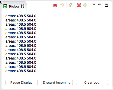
In this case the program is only looking at the array of areas, but in a real example all the values would more likely be used. Using the Riolog in VS Code or the Driver Station log you can see the values as they are retrieved. This program is using a sample static image so they areas don’t change, but you can imagine with a camera on your robot, the values would be changing constantly.
Path Planning
Path Planning is the process of creating and following trajectories. These paths use the WPILib trajectory APIs for generation and a Ramsete Controller for following. This section highlights the process of characterizing your robot for system identification, trajectory following and usage of PathWeaver. Users may also want to read the generic trajectory following documents for additional information about the API and non-commandbased usage.
Notice on Swerve Support
Swerve support in path following has a couple of limitations that teams need to be aware of: - WPILib currently does not support swerve in simulation, please see this pull request. - SysID only supports tuning the swerve heading using a General Mechanism project and does not regularly support module velocity data. A workaround is to lock the module’s heading into place. This can be done via blocking module rotation using something like a block of wood. - Pathweaver and Trajectory following currently do not incorporate independent heading. Path following using the WPILib trajectory framework on swerve will be the same as a DifferentialDrive robot.
We are sorry for the inconvenience.
Robot Characterization
Introduction to Robot Characterization
The characterization tools consist of an application that runs on the user’s PC and matching robot code that runs on the user’s robot. The PC application will send control signals to the robot over NetworkTables, while the robot sends data back to the application. The application then processes the data and determines characterization parameters for the user’s robot mechanism, as well as producing diagnostic plots. Data can be saved (in JSON format) for future use, if desired.
What is “Characterization?”
“Characterization” - or, more formally, system identification - is the process of determining a mathematical model for the behavior of a system through statistical analysis of its inputs and outputs.
In FRC, the most common system that we’re interested in characterizing is the permanent-magnet DC motor. In particular, we’re interested in figuring out which motor input (i.e. voltage from the motor controller) is required to achieve our desired outputs (i.e. velocity and acceleration of the motor).
Fortunately, it is not so difficult to do this. A permanent-magnet DC motor (with no load other than friction and inertia) will obey the following “voltage-balance equation” (for more information, see this paper):
where \(V\) is the applied voltage, \(d\) is the displacement (position) of the motor, \(\dot{d}\) is its velocity, and \(\ddot{d}\) is its acceleration (the “overdot” notation traditionally denotes the derivative with respect to time).
Heuristically, we can interpret the coefficients in the above equation as follows:
kS is the voltage needed to overcome the motor’s static friction, or in other words to just barely get it moving; it turns out that this static friction (because it’s, well, static) has the same effect regardless of velocity or acceleration. That is, no matter what speed you’re going or how fast you’re accelerating, some constant portion of the voltage you’ve applied to your motor (depending on the specific mechanism assembly) will be going towards overcoming the static friction in your gears, bearings, etc; this value is your kS. Note the presence of the signum function, because friction force always opposes the direction-of-motion.
kV describes how much voltage is needed to hold (or “cruise”) at a given constant velocity while overcoming the electromagnetic resistance in the motor and any additional friction that increases with speed (known as viscous drag). The relationship between speed and voltage (at constant acceleration) is almost entirely linear (with FRC® components, anyway) because of how permanent-magnet DC motors work.
kA describes the voltage needed to induce a given acceleration in the motor shaft. As with kV, the relationship between voltage and acceleration (at constant velocity) is almost perfectly linear for FRC components.
Once these coefficients have been determined (here accomplished by a multiple linear regression), we can then take a given desired velocity and acceleration for the motor and calculate the voltage that should be applied to achieve it. This is very useful - not only for, say, following motion profiles, but also for making mechanisms more controllable in open-loop control, because your joystick inputs will more closely match the actual mechanism motion.
Some of the tools in this toolsuite introduce additional terms into the above equation to account for known differences from the simple case described above - details for each tool can be found below:
Included Characterization Tools
Note
Many other types of mechanisms can be characterized by simply adapting the existing code in this library.
The robot characterization toolsuite currently supports characterization for:
Simple Motor Setups
Drivetrains
Arms
Elevators
The simple motor characterization tool determines the best-fit parameters for the equation:
where \(V\) is the applied voltage, \(d\) is the displacement (position) of the drive, \(\dot{d}\) is its velocity, and \(\ddot{d}\) is its acceleration. This is the model for a permanent-magnet dc motor with no loading other than friction and inertia, as mentioned above, and is an accurate model for flywheels, turrets, and horizontal linear sliders.
The drivetrain characterization tool determines the best-fit parameters for the equation:
where \(V\) is the applied voltage, \(d\) is the displacement (position) of the drive, \(\dot{d}\) is its velocity, and \(\ddot{d}\) is its acceleration. This is the same modeling equation as is used in the simple motor characterization - however, the drivetrain characterizer is specifically set up to run on differential drives, and will characterize each side of the drive independently if desired.
The drivetrain characterizer can also determine the effective trackwidth of your robot using a gyro. More information on how to run the characterization is available in the track width characterization article.
The arm characterization tool determines the best-fit parameters for the equation:
where \(V\) is the applied voltage, \(\theta\) is the angular displacement (position) of the arm, \(\dot{\theta}\) is its angular velocity, and \(\ddot{\theta}\) is its angular acceleration. The cosine term (\(kCos\)) is added to correctly account for the effect of gravity.
The elevator characterization tool determines the best-fit parameters for the equation:
where \(V\) is the applied voltage, \(d\) is the displacement (position) of the drive, \(\dot{d}\) is its velocity, and \(\ddot{d}\) is its acceleration. The constant term (\(kG\)) is added to correctly account for the effect of gravity.
Installing the System Identification Tool
The system identification tool (also referred to as sysid) is included with the WPILib Installer.
Note
The old Python characterization tool from previous years is no longer supported.
Launching the System Identification Tool
The system identification tool can be opened from the Start Tool option in VS Code or by using the shortcut inside the WPILib Tools desktop folder (Windows).
Configuring a Project
To use the toolsuite, we first need to configure the settings for your specific mechanism.
Configure Project Parameters
In order to run on your robot, the tool must know some parameters about how your robot is set up.
First, you need to use the Analysis Type field to select the appropriate project config. General Mechanism is for non-drivetrain mechanisms (e.g. Simple Motor, Arm, Elevator), Drivetrain is for Drivetrain mechanisms, and Romi is for the Romi robots. This allows you to fill out the parameters specific to the type of system you are using.
The rest of the Generator widget is focused on the proper settings based off of the analysis type:
The Motor / Motor Controller Selection allows you to add ports for each motor controller that will be used. The + and - buttons let you add and remove ports respectively.
Note
If you are plugging in your encoders into motor controllers make sure that the motor controller type and port(s) are the first ones you specify.
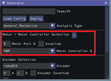
Each motor port contains the following parts:
Motor Port is where you add the port number for a specific controller
Inverted should be checked if the motorcontroller should be inverted
Motor Controller is the type of motor controller that will be used.
The Encoder Selection allows you to configure the encoders that will be used. The types of encoder you can use will vary with the first motor controller type specified (see note above).
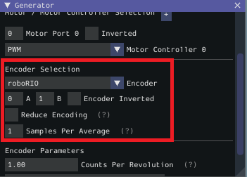
General Types (consistent across all motor controller selections):
roboRIOcorresponds to any encoders that are plugged into the roboRIO,CANCodercorresponds to the CTRE CANCoder.TalonSRX:
Built-incorresponds to any quadrature encoder plugged into the encoder port,Tachometercorresponds to the CTRE Tachometer plugged into the encoder port.TalonFX:
Built-incorresponds to the integrated encoder on the TalonFX motor.Spark MAX:
Encoder Portrefers to an encoder plugged into the encoder port,Data Portrefers to an encoder plugged into the data port.Venom:
Built-inrefers to an encoder plugged into the Venom’s encoder port.
Here are the following settings that can be configured (although the settings that are visible will vary by the previously selected encoder type):
Ports (either A and B or CANCoder Port
Encoder Inverted should be checked if a positive motor power doesn’t correspond to a positive increase in encoder values
Samples Per Average is how many samples will be averaged per velocity measurement. A value greater than one can help reduce encoder noise and 5-10 is recommended for encoders with high CPR. Only mess with this setting if a previous run of SysId resulted in extremely noisy data.
Reduce Encoding should be checked if using high resolution encoders (e.g. CTRE Mag Encoders or REV Through Bore Encoder) that are plugged into the roboRIO. Do note, that if this is checked, you will have to update your team’s robot code to also reduce encoding.
Time Measurement Window is the period of time in milliseconds that the velocity measurement will be taken across. This setting can reduce measurement lag at the cost of possibly introducing more noise. Only modify this if data lag is impeding accurate control and data collection.
Counts Per Revolution is the encoder counts per revolution for your encoder which is generally specified on a datasheet. Common values include:
CTRE Magnetic Encoder: 4096
Falcon 500 Integrated: 2048
REV Throughbore: 8192
NEO (and NEO 550) Integrated Encoders (REV already handles this value): 1
Gearing is the gearing between the encoder and output shaft. For example, an magnetic encoder on a kit chassis would have a gearing of one as it is on a 1:1 ratio with the output shaft. However, if is was an integrated encoder in a motor that was in the gearbox, the gearing would be 10.71 (per Andymark) since there is now gearing between the encoder and the output shaft.
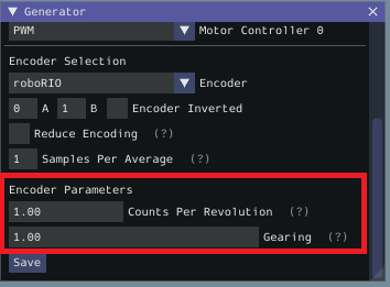
Gyro lets you select the type of supported gyro. Gyro Parameter lets you configure additional settings needed to configure the previously specified gyro.
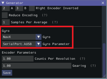
Loading and Saving Configurations
Once your robot configuration is set, you may save it to a location/name of your choice with the Save button:
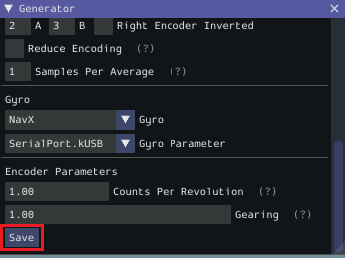
Accordingly, you can also load an existing config file with the Load Config button:
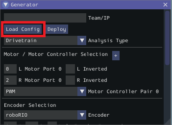
Deploying Project
Once your project has been configured, it’s time to deploy the robot project to run the characterization routine.
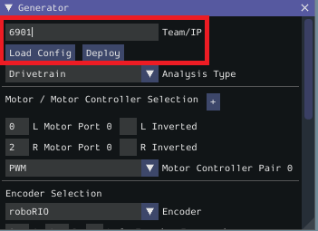
Team/IP is where you set your team number or IP. You can then deploy the code with the Deploy label.
Running the Characterization Routine
Once the characterization code has been deployed, we can now run the characterization routine, and record the resulting data for analysis.
Note
Ensure you have sufficient space around the robot before running any characterization routine! The drive characterization requires at least 10’ of space, ideally closer to 20’. The robot drive can not be accurately characterized while on blocks.
Connect to the Robot
Next, we must connect to the robot. Select “Client” at the top of the Logger window and enter your team number. To characterize a simulated robot program, you can type in localhost. Finally, press the Apply button. The NetworkTables connection indicator will be visible next to the Apply button.
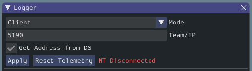
If the tool does not seem to be successfully connecting, try rebooting the robot. Eventually, the status should change to NT Connected, indicating the tool is successfully communicating with the robot.
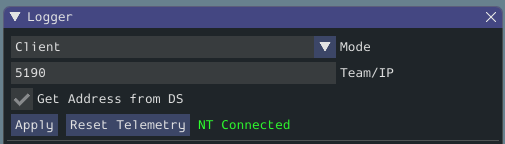
Project Parameters
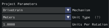
Mechanism controls what data is sampled and how gravity is expected to affect the analysis.
Unit Type is the units you are using and the units that SysID will export the gains in.
Units Per Rotation defines anything that affects the change from rotations of the output shaft to the units selected above. As an example say you are using a KOP chassis and units of meters. The gearing is already accounted for in the generator. We have to take into account how our wheel will change the distance we have traveled per rotation. The standard chassis has 6” (0.1524 meters) diameter wheels, so to get the circumference we need to multiply by Pi. The calculation looks like:
Voltage Parameters
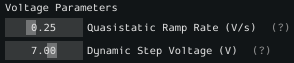
Quasistatic Ramp Rate controls how quickly the voltage will ramp up during the quasistatic tests. The goal here is to get the voltage ramped up enough that a trend emerges. If the amount of space you have to run the robot is small you might need to slightly increase this ramp rate.
Dynamic Step Voltage is the voltage that will be applied immediately on start to determine how your robot accelerates. If your robot is short on space you should slightly reduce the voltage.
Running Tests
A standard motor characterization routine consists of two types of tests:
Quasistatic: In this test, the mechanism is gradually sped-up such that the voltage corresponding to acceleration is negligible (hence, “as if static”).
Dynamic: In this test, a constant ‘step voltage’ is given to the mechanism, so that the behavior while accelerating can be determined.
Each test type is run both forwards and backwards, for four tests in total, corresponding to the four buttons.
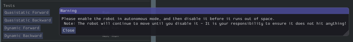
The tests can be run in any order, but running a “backwards” test directly after a “forwards” test is generally advisable (as it will more or less reset the mechanism to its original position).
Follow the instructions in the pop-up windows after pressing each test button.
You can determine the track width of the robot by selecting the Drivetrain (Angular) test. This will also provide angular Kv and Ka parameters.
This test will spin your robot to determine an empirical trackwidth. It compares how far the wheel encoders drove against the reported rotation from the gyroscope. To get the best results your wheels should maintain contact with the ground.
Note
For high-friction wheels (like pneumatic tires), the empirical trackwidth calculated by sysid may be significantly different from the real trackwidth (e.g., off by a factor of 2). The empirical value should be preferred over the real one in robot code.
The entire routine should look something like this:
After all four tests have been completed, you can select the folder location for the save file and click Save.
This will save the data as a JSON file with the specified location/name. A timestamp (%Y%m%d-%H%M) will be appended to the chosen filename. Additionally, the name of the file saved will be shown in the Program Log.
Note
The number of samples collected for each test will be displayed in the Program Log.
Analyzing Data
Important
WPILib standarizes on SI units, so its recommended that the Units option is set to Meters.
Once we have data from a characterization run, we can analyze it using the Analyzer and Diagnostic Plots widgets.
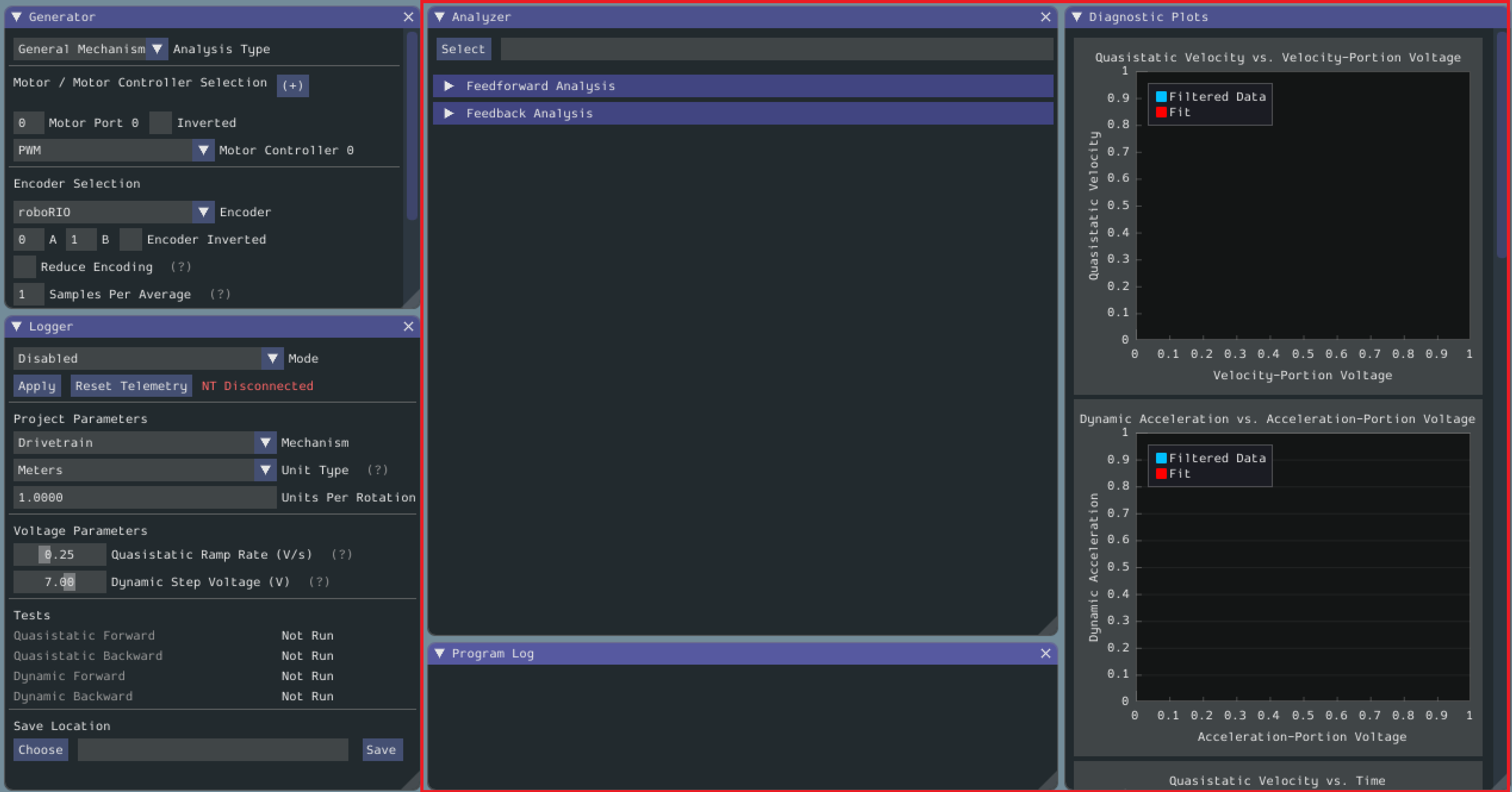
Loading your Data File
Now it’s time to load the data file we saved from the logger tool. Click on Select.
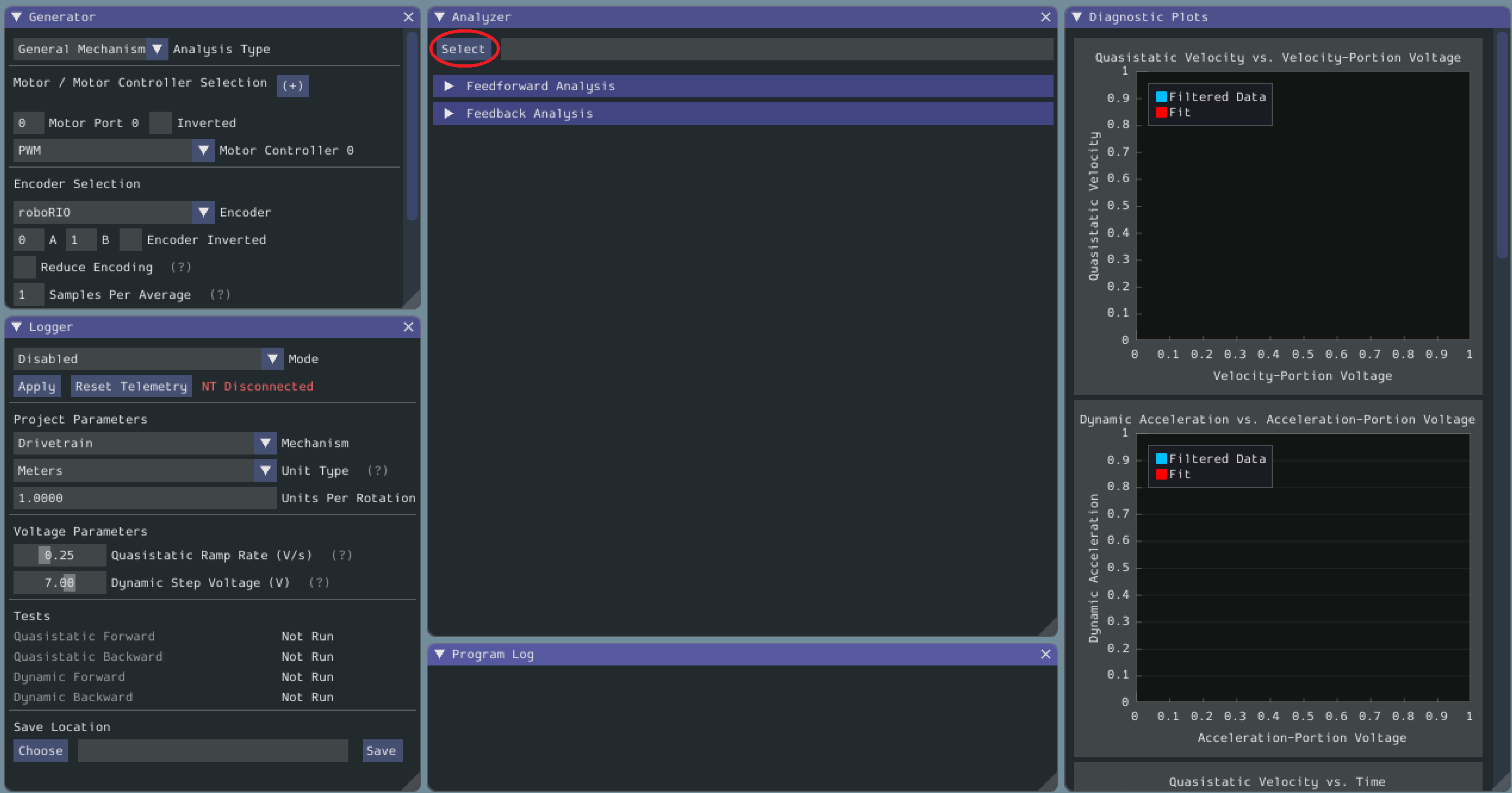
In the resulting file dialog, select the JSON file you want to analyze. If the file appears to be malformed, an error will be shown.
Running Feedforward Analysis
Click the dropdown arrow on the Feedforward Section.
Note
If you would like to change units, you will have to press the Override Units button and fill out the information on the popup.
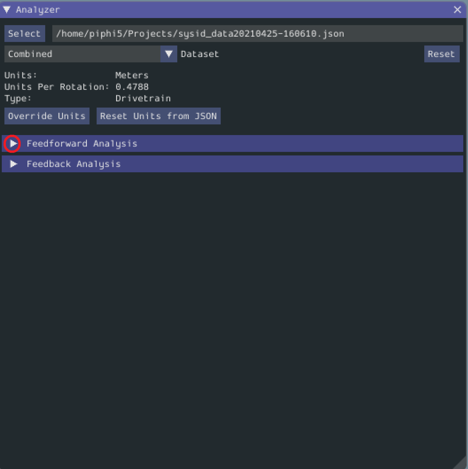
By default, the analysis will be run by combining all the data in the test. For a finer-grained analysis, the analysis may be limited to a specific subset of data using the subset dropdown menu.
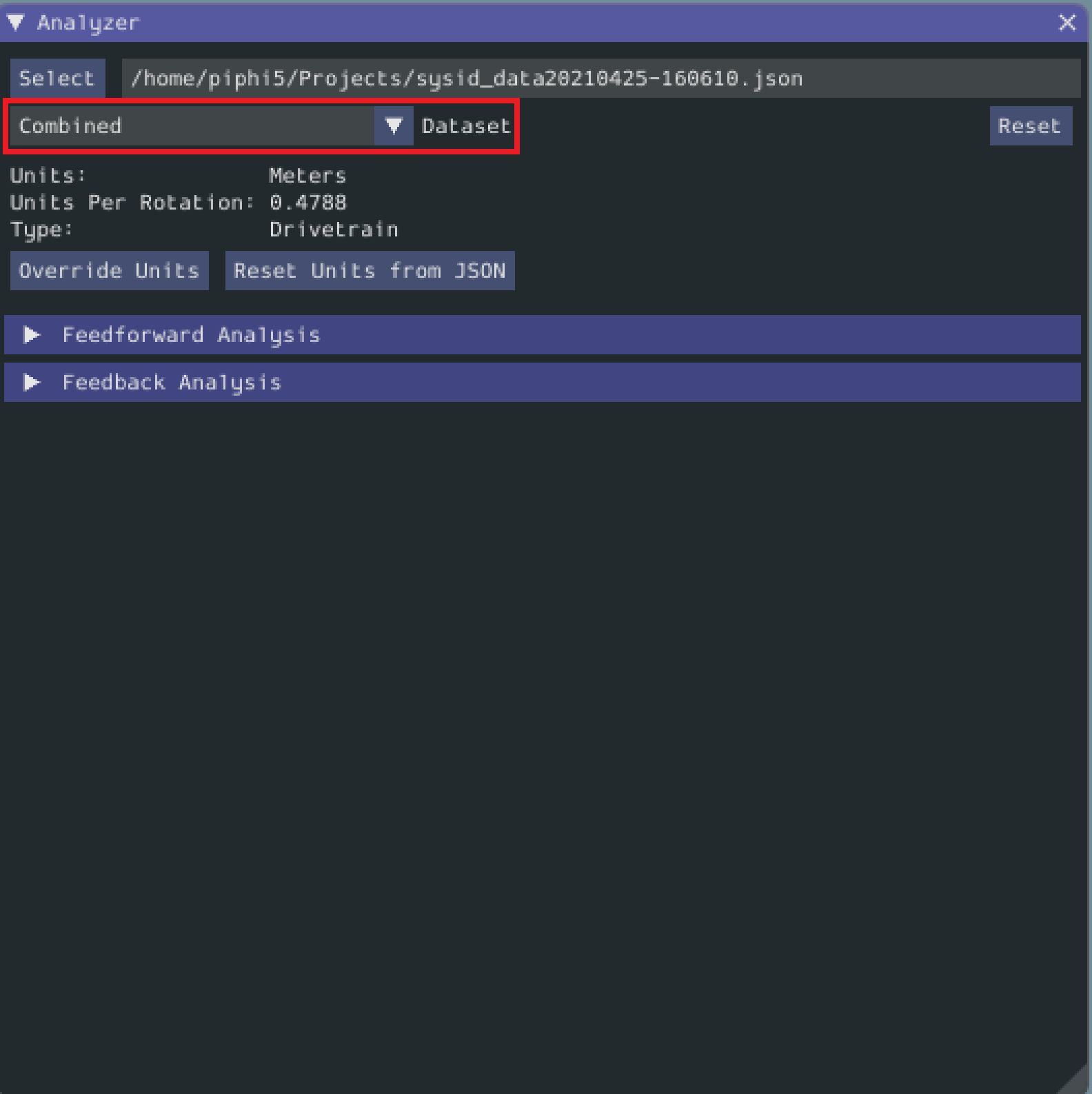
The computed coefficients of the mechanism characterization will then be displayed.
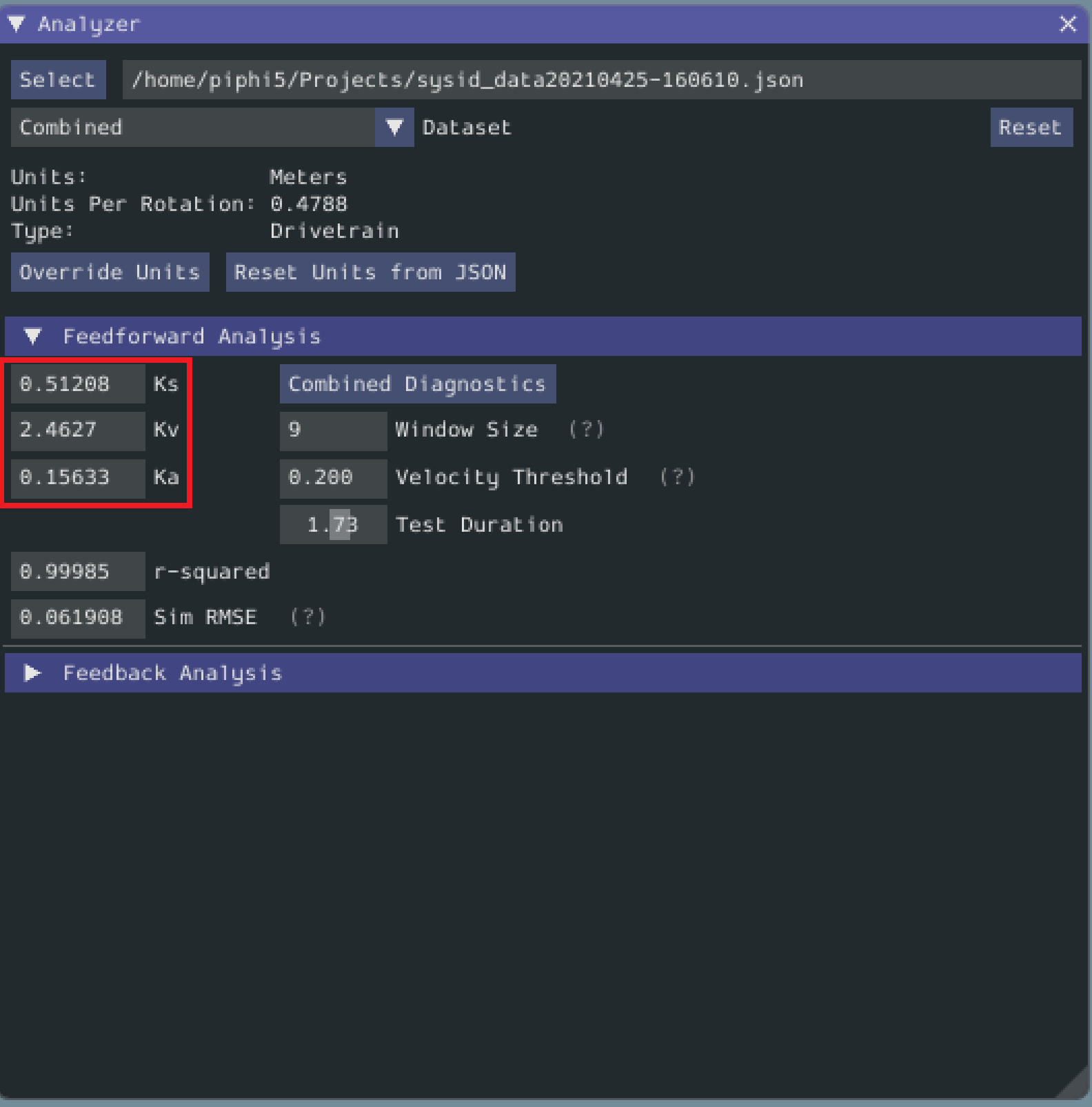
There are also two accuracy metrics that are computed with this tool: r-squared and RMSE. The r-squared metric refers to the goodness of fit of the tool’s OLS (Ordinary Least Squares) fit. The RMSE (Root Mean Squared Error) is the error (in the measured units) between the collected velocities and the predicted velocities from a simulation based on the feedforward gains.
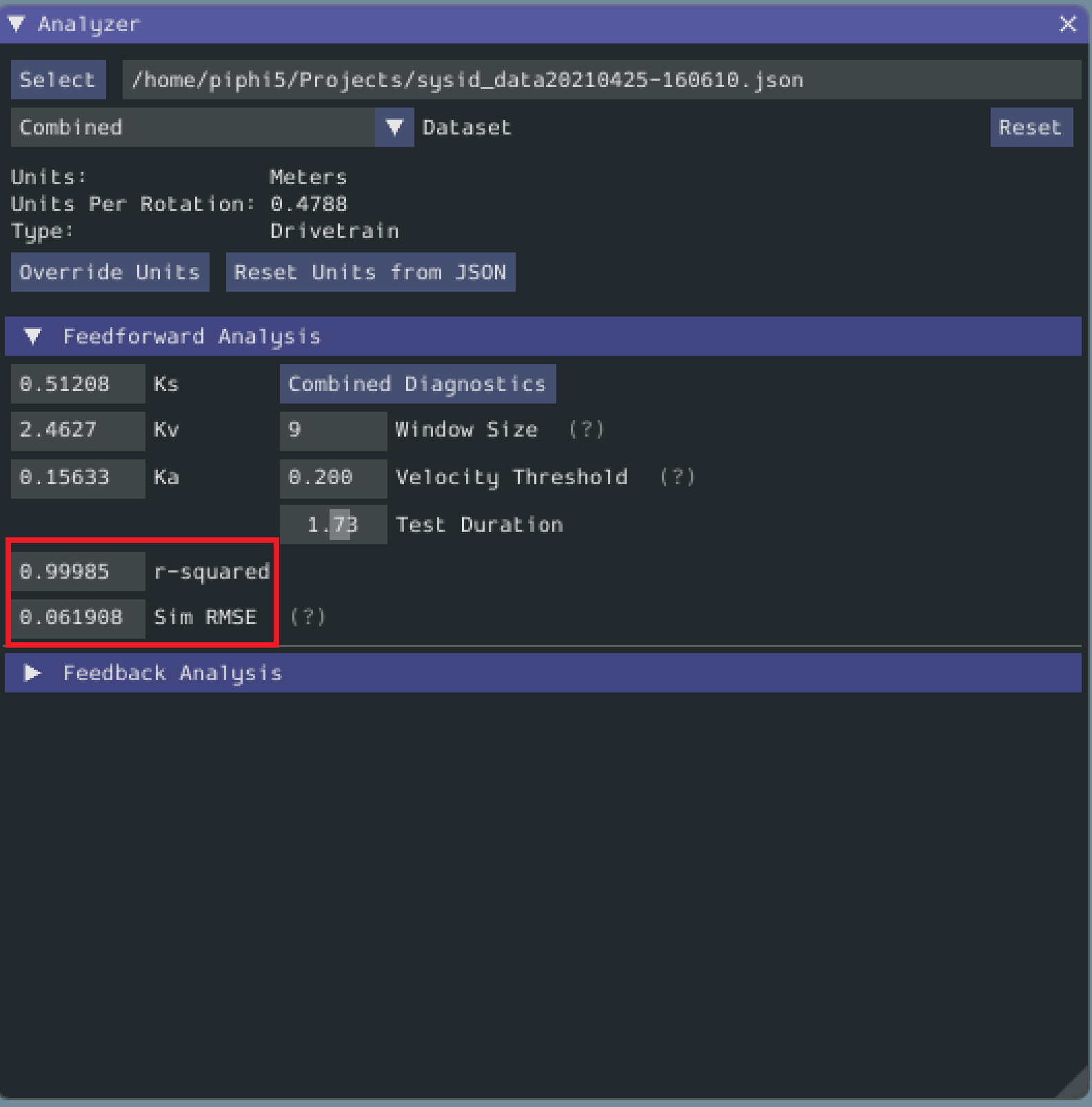
Viewing Diagnostics
The first diagnostic to look at is the r-squared - it should be somewhere north of ~.9. If it is significantly lower than this, there is likely a problem with your characterization data.
The next diagnostic to look at is the RMSE to make sure that the error is reasonable and within your desired constraints.
To investigate further, you can look at several diagnostic plots on the side.
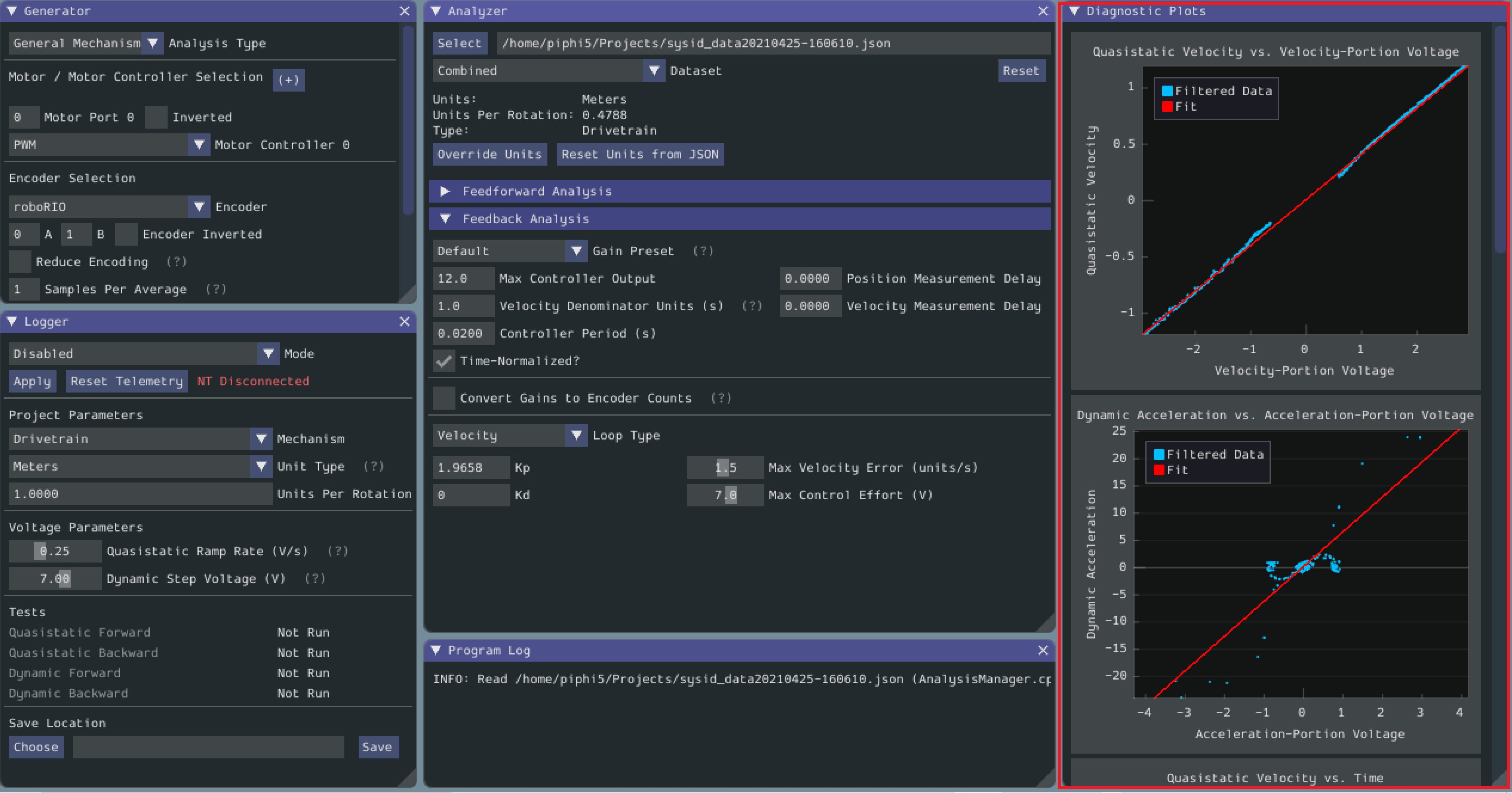
Time-Domain Diagnostics
The Time-Domain Diagnostics plots display velocity and acceleration versus time over the course of the analyzed tests. These should look something like this (other mechanisms will be highly similar):
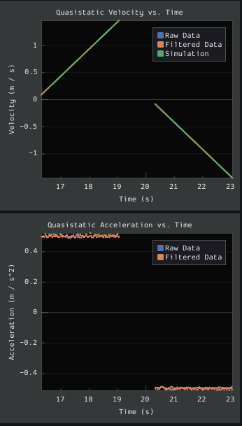
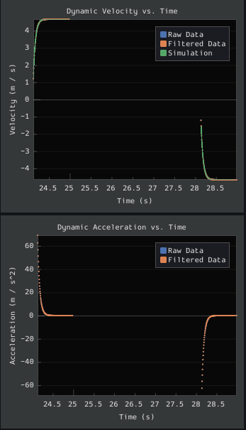
Note
There may be mirroring across the x axis for the drivetrain test. That is normal and is simply the result of the left- and right-side encoders having different signs - this does not cause any trouble for the characterization tool.
The velocity time domain plots contain three sets of data: Raw Data, Filtered Data, and Simulation. The Raw Data is the recorded data from your robot, the Filtered Data is the data after a median filter has been applied to the data, and the Simulation represents the velocity predictions of a model based off of the feedforward gains from the tool. The acceleration graphs only contain the Raw Data and Filtered Data.
The quasistatic test ought to have nearly linear velocity, and nearly-zero acceleration (hense “quasistatic”). The dynamic test ought to have velocity that asymptotically approaches a steady-state speed (the shape of the curve should be exponential, in fact), and acceleration that, accordingly, rapidly falls to zero (also exponentially, as the derivative of an exponential function is also an exponential function).
Deviation from this behavior is a sign of an error, either in your robot setup, analysis settings, or your test procedure.
Voltage-Domain Diagnostics
The Voltage-Domain Diagnostics plots velocity and acceleration versus voltage. Velocity is ploted for the quasistatic test, and acceleration is plotted for the dynamic test. For a typical drive characterization, the plots should resemble this (again, other mechanisms will be similar)
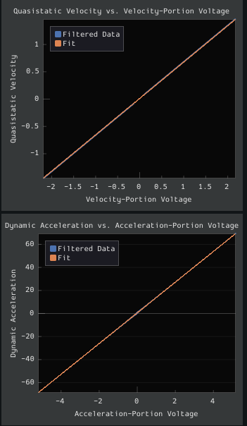
Both plots should be linear, however the dynamic plot will almost certainly have substantially-more noise. The noise on the dynamic plot may be reduced by increasing the Window Size setting.
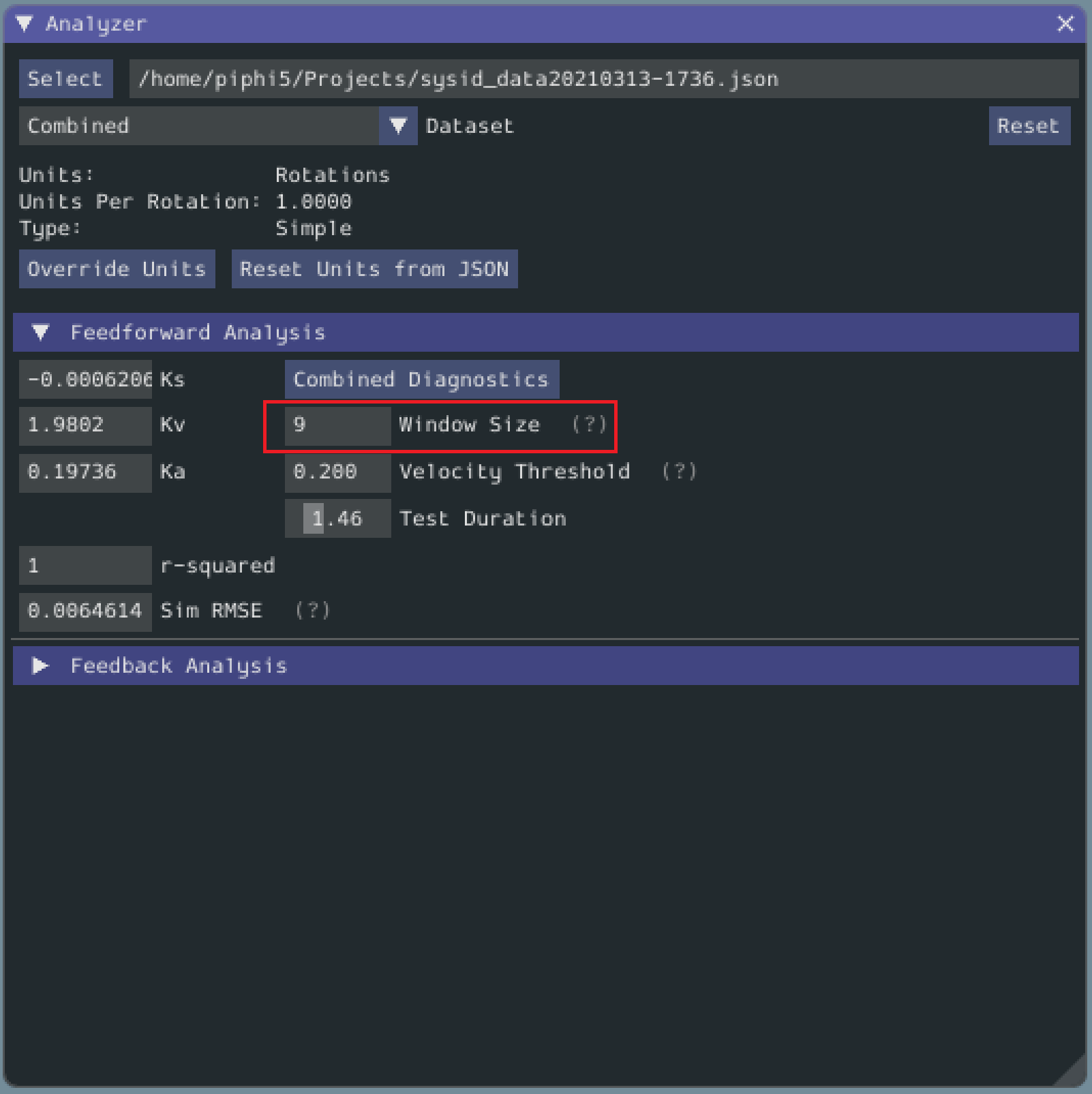
However, if your robot or mechanism has low mass compared to the motor power, this may “eat” what little meaningful acceleration data you have (however, in these cases kA will tend towards zero and can usually be ignored, anyway).
Note
The x-axis corresponds to velocity-portion voltage and acceleration-portion voltage, respectively - as the governing voltage-balance equations are multi-dimensional, plots against raw voltage are not as useful as one might expect.
When something has gone wrong with the characterization, diagnostic plots and console output provide crucial clues as to what has gone wrong. This section describes some common failures encountered while running the characterization tool, the identifying features of their diagnostic plots, and the steps that can be taken to fix them.
One of the most-common errors is an inappropriate value for the motion threshold.
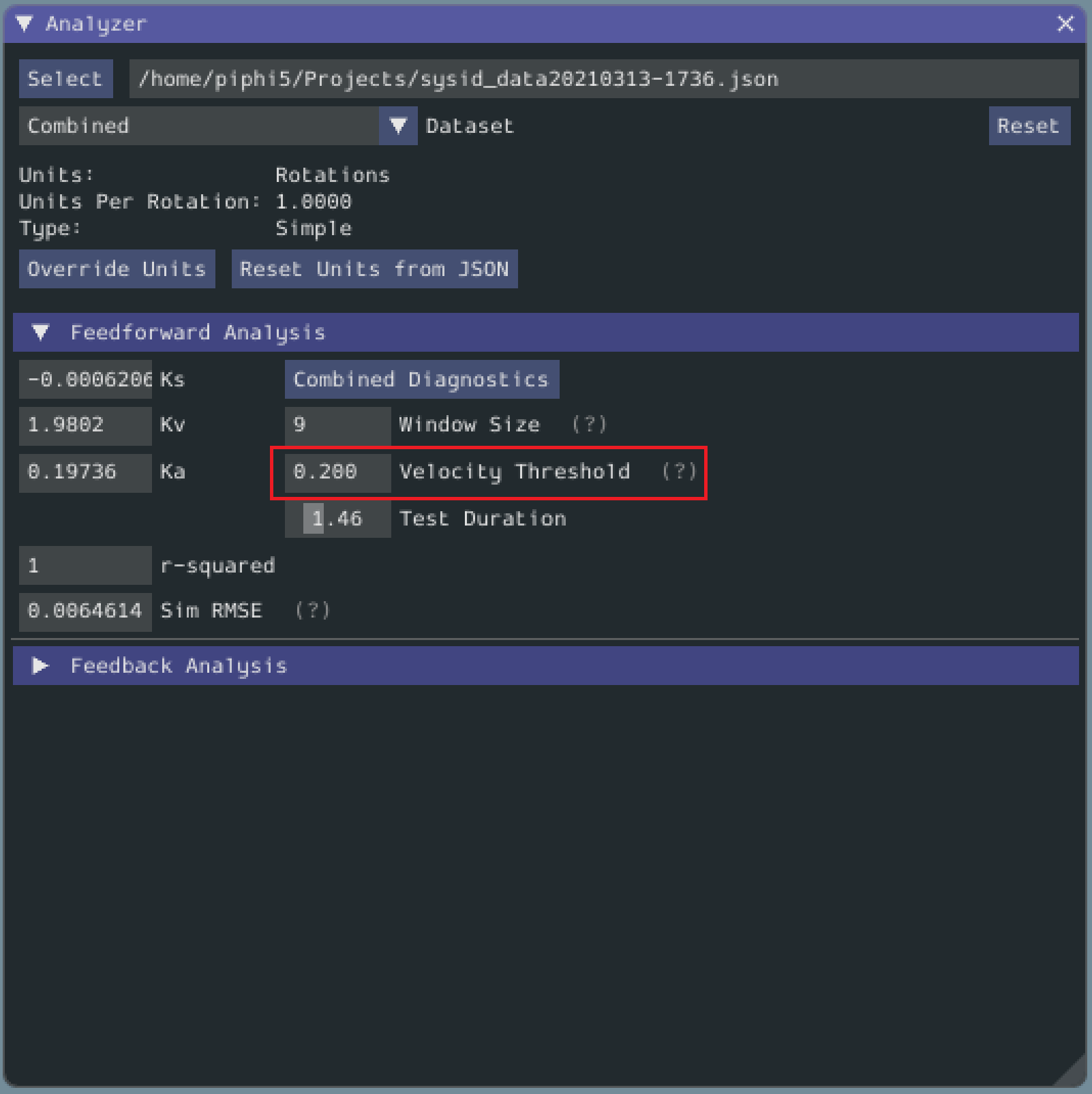
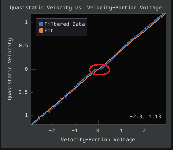
The presence of a “leading tail” (emphasized by added red circle) on the voltage-domain plots indicates that the Motion Threshold setting is too low, and thus data points from before the robot begins to move are being included.
To solve this, increase the setting and re-analyze the data.
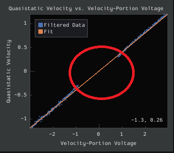
While not nearly as problematic as a too-low threshold, a motion threshold that is too high will result in a large “gap” in the voltage domain quasistatic plot.
To solve this, decrease the setting and re-analyze the data.
If the dynamic test is run too long, it tends to accumulate data that will only skew the kA fit. This is noticeable with a large concentration of points towards the middle of the Voltage Domain Acceleration plot. This issue can be assisted by decreasing the Test Duration slider.
Magnetic encoders such as the CTRE Mag Encoder and the AndyMark magnetic encoder are extremely popular in FRC. However, a particular noise pattern has been observed when these encoders are used on robot drives, whose particular cause is not yet known. This noise pattern is uniquely distinguished by significant velocity noise proportional to motor velocity, and is particularly common on the kit-of-parts toughbox mini gearboxes.
Characterization constants can sometimes be accurately determined even from data polluted this noise by increasing the window size setting. However, this sort of encoder noise is problematic for robot code much the same way it is problematic for the characterization tool. As the root cause of the noise is not known, it is recommended to try a different encoder setup if this is observed, either by moving the encoders to a different shaft, replacing them with a different type of encoder, or increasing the sample per average in project generation (adds an additional layer of filtering).
Feedback Analysis
Important
These gains are, in effect, “educated guesses” - they are not guaranteed to be perfect, and should be viewed as a “starting point” for further tuning.
To view the feedback constants, click on the dropdown arrow on the Feedback section.

This view can be used to calculate optimal feedback gains for a PD or P controller for your mechanism (via LQR).
Enter Controller Parameters
Note
The “Spark Max” preset assumes that the user has configured the controller to operate in the units of analysis with the SPARK MAX API’s position/velocity scaling factor feature.
The calculated feedforward gains are dimensioned quantities. Unfortunately, not much attention is often paid to the units of PID gains in FRC® controls, and so the various typical options for PID controller implementations differ in their unit conventions (which are often not made clear to the user).
To specify the correct settings for your PID controller, use the following options.
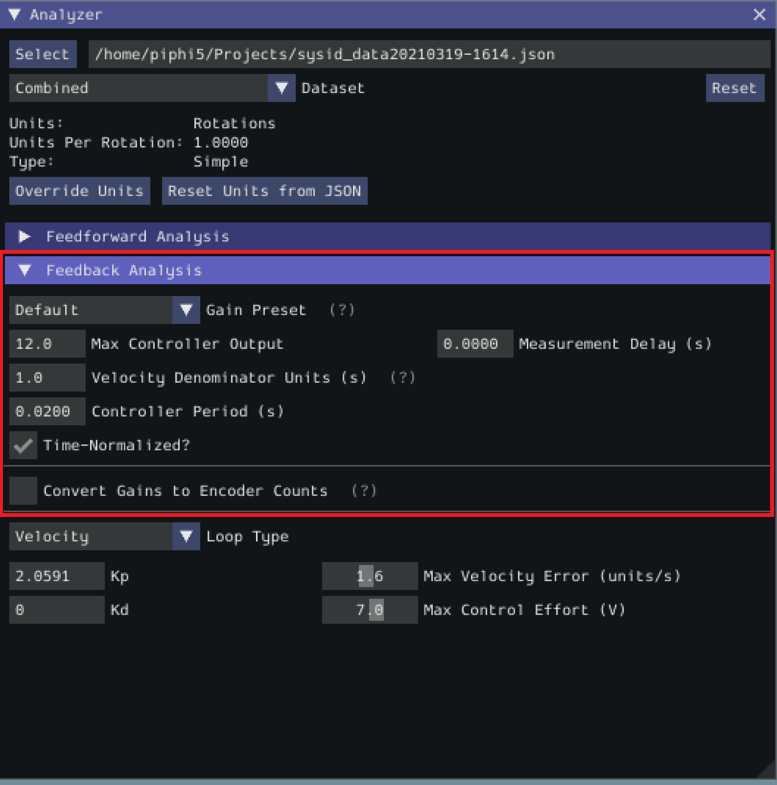
Gain Settings Preset This drop-down menu will auto-populate the remaining fields with likely settings for one of a number of common FRC controller setups. Note that some settings, such as post-encoder gearing, PPR, and the presence of a follower motor must still be manually specified (as the analyzer has no way of knowing these without user input), and that others may vary from the given defaults depending on user setup.
Controller Period This is the execution period of the control loop, in seconds. The default RIO loop rate is 50Hz, corresponding to a period of 0.02s. The onboard controllers on most “smart controllers” run at 1Khz, or a period of 0.001s.
Max Controller Output This is the maximum value of the controller output, with respect to the PID calculation. Most controllers calculate outputs with a maximum value of 1, but Talon controllers have a maximum output of 1023.
Time-Normalized Controller This specifies whether the PID calculation is normalized to the period of execution, which affects the scaling of the D gain.
Controller Type This specifies whether the controller is an onboard RIO loop, or is running on a smart motor controller such as a Talon or a SPARK MAX.
Post-Encoder Gearing This specifies the gearing between the encoder and the mechanism itself. This is necessary for control loops that do not allow user-specified unit scaling in their PID computations (e.g. those running on Talons). This will be disabled if not relevant.
Encoder EPR This specifies the edges-per-revolution (not cycles per revolution) of the encoder used, which is needed in the same cases as Post-Encoder Gearing.
Has Follower Whether there is a motor controller following the controller running the control loop, if the control loop is being run on a peripheral device. This changes the effective loop period.
Follower Update Period The rate at which the follower (if present) is updated. By default, this is 100Hz (every 0.01s) for the Talon SRX, Talon FX, and the SPARK MAX, but can be changed.
Note
If you select a smart motor controller as the preset (e.g. TalonSRX, SPARK MAX, etc.) the Convert Gains checkbox will be automatically checked. This means the tool will convert your gains so that they can be used through the smart motor controller’s PID methods. Therefore, if you would like to use WPILib’s PID Loops, you must uncheck that box.
Note
If you are using default smart motor controller settings or WPILib PID Control without additional filtering, SysId handles this for you.
Many “smart motor controllers” (such as the Talon SRX, Venom, Talon FX, and SPARK MAX) apply substantial low-pass filtering to their encoder velocity measurements, which can introduce a significant amount of phase lag. This can cause the calculated gains for velocity loops to be unstable. This can be accounted for with the Measurement Delay box.
However, the measurement delays have already been calculated for the default settings of the previously mentioned motor controllers so for most users this is handled by selecting the right preset in Gain Settings Preset.
The following only applies if the user decides to implement their own custom filtering settings (e.g. adding a moving average filter to a WPILib PID loop or changing smart motorcontroller measurement period and/or measurement window size) as the measurement delay must be recalculated. Here is the general formula that can be used for filters with moving windows (e.g. median filter + moving average filter):
Where T is the period at which measurements are sampled (RIO default is 20 ms) and n is the size of the moving window used.
Specify Optimality Criteria
Finally, the user must specify what will be considered an “optimal” controller. This takes the form of desired tolerances for the system error and control effort - note that it is not guaranteed that the system will obey these tolerances at all times.
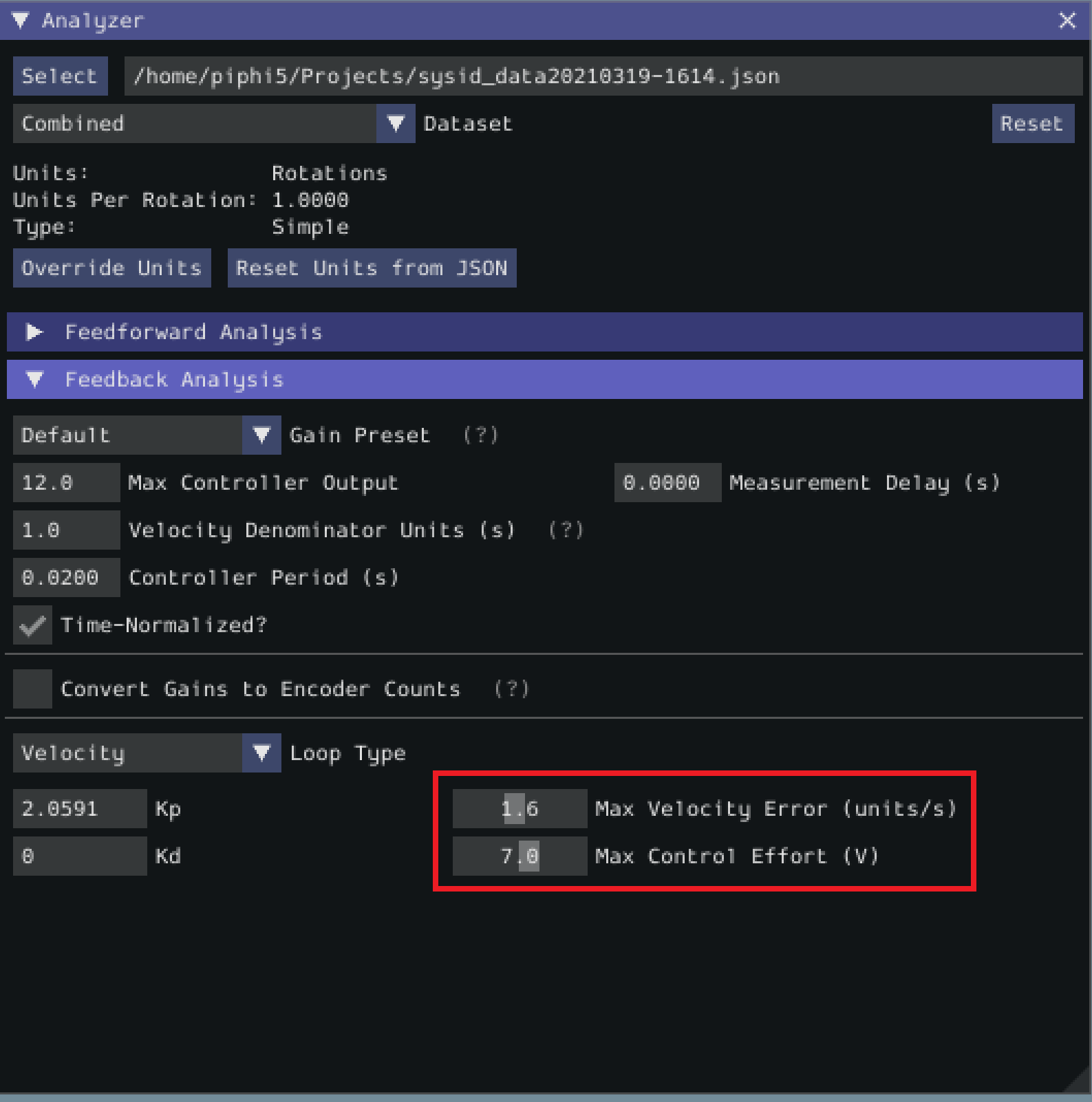
As a rule, smaller values for the Max Acceptable Error and larger values for the Max Acceptable Control Effort will result in larger gains - this will result in larger control efforts, which can grant better setpoint-tracking but may cause more violent behavior and greater wear on components.
The Max Acceptable Control Effort should never exceed 12V, as that corresponds to full battery voltage, and ideally should be somewhat lower than this.
Select Loop Type
It is typical to control mechanisms with both position and velocity PIDs, depending on application. Either can be selected using the drop-down Loop Type menu.
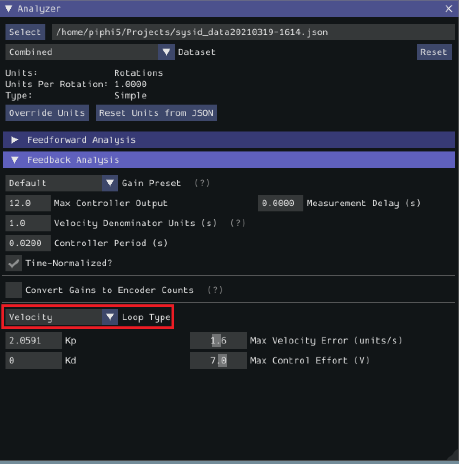
Additional Utilities and Tools
This page mainly covers useful information about additional functionality that this tool provides.
JSON Converters
There are a two JSON Utility tools that can be used in the JSON Converters tab: FRC-Char Converter and JSON to CSV Converter.
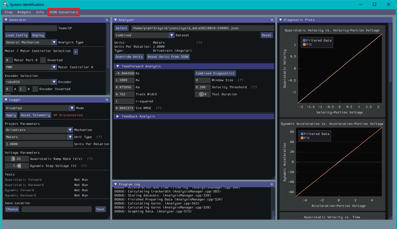
The FRC-Char Converter reads in an FRC-Char JSON and converts it into a SysId JSON that the tool can read.
The JSON to CSV Converter takes a SysId JSON and outputs a CSV file. If the JSON had Drivetrain Mechanism data, the columns are: Timestamp (s), Test, Left Volts (V) , Right Volts (V), Left Position ({0}), Right Position ({units}), Left Velocity ({units}/s), Right Velocity ({units}/s), Gyro Position (deg), Gyro Rate (deg/s).
If the JSON had General Mechanism data, the CSV has the following columns: Timestamp (s), Test, Volts (V), Position({units}), Velocity ({units}/s).
ImGui Tips
The following are essentially handy features that come with the ImGui framework that SysId uses:
To add or remove certain data from the plots, click on the color of the data that you would like to hide or remove.
For example, if we want to hide sim data, we can click the green color box.
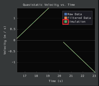
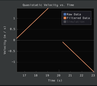
If you zoom in to plots and want to revert back to the normally sized plots, just double click on the plot and it will automatically resize it.
Here is a plot that is zoomed in:
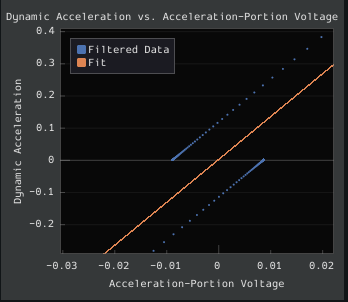
After double clicking, it is automatically resized:
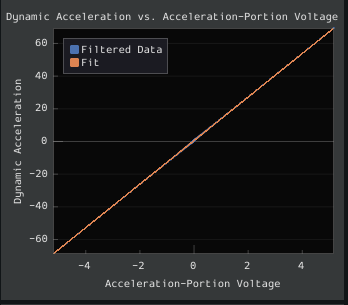
To set the value of a slider as a number rather than sliding the widget, you can CTRL + Click the slider and it will allow you to input a number.
Here is a regular slider:
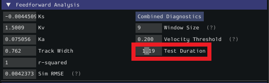
Here is the input after double clicking the slider:
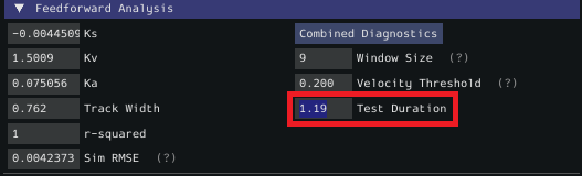
Trajectory Tutorial
This is full tutorial for implementing trajectory generation and following on a differential-drive robot. The full code used in this tutorial can be found in the RamseteCommand example project (Java, C++).
Trajectory Tutorial Overview
Note
Before following this tutorial, it is helpful (but not strictly necessary) to have a baseline familiarity with WPILib’s PID control, feedforward, and trajectory features.
Note
The robot code in this tutorial uses the command-based framework. The command-based framework is strongly recommended for beginning and intermediate teams.
The goal of this tutorial is to provide “end-to-end” instruction on implementing a trajectory-following autonomous routine for a differential-drive robot. By following this tutorial, readers will learn how to:
Accurately characterize their robot’s drivetrain to obtain accurate feedforward calculations and approximate feedback gains.
Configure a drive subsystem to track the robot’s pose using WPILib’s odometry library.
Generate a simple trajectory through a set of waypoints using WPILib’s
TrajectoryGeneratorclass.Follow the generated trajectory in an autonomous routine using WPILib’s
RamseteCommandclass with the calculated feedforward/feedback gains and pose.
This tutorial is intended to be approachable for teams without a great deal of programming expertise. While the WPILib library offers significant flexibility in the manner in which its trajectory-following features are implemented, closely following the implementation outlined in this tutorial should provide teams with a relatively-simple, clean, and repeatable solution for autonomous movement.
The full robot code for this tutorial can be found in the RamseteCommand Example Project (Java, C++).
Why Trajectory Following?
FRC® games often feature autonomous tasks that require a robot to effectively and accurately move from a known starting location to a known scoring location. Historically, the most common solution for this sort of task in FRC has been a “drive-turn-drive” approach - that is, drive forward by a known distance, turn by a known angle, and drive forward by another known distance.
While the “drive-turn-drive” approach is certainly functional, in recent years teams have begun tracking smooth trajectories which require the robot to drive and turn at the same time. While this is a fundamentally more-complicated technical task, it offers significant benefits: in particular, since the robot no longer has to stop to change directions, the paths can be driven much faster, allowing a robot to score more game pieces during the autonomous period.
Beginning in 2020, WPILib now supplies teams with working, advanced code solutions for trajectory generation and tracking, significantly lowering the “barrier-to-entry” for this kind of advanced and effective autonomous motion.
Required Equipment
To follow this tutorial, you will need ready access to the following materials:
A differential-drive robot (such as the AndyMark AM14U4), equipped with:
Quadrature encoders for measuring the wheel rotation of each side of the drive.
A gyroscope for measuring robot heading.
A driver-station computer configured with:
Step 1: Characterizing Your Robot Drive
Note
For detailed instructions on using the System Identification tool, see its dedicated documentation.
Note
The drive characterization process requires ample space for the robot to drive. Be sure to have at least a 10’ stretch (ideally closer to 20’) in which the robot can drive during the characterization routine.
Note
The characterization data for this tutorial has been generously provided by Team 5190, who generated it as part of a demonstration of this functionality at the 2019 North Carolina State University P2P Workshop.
Before accurately following a path with a robot, it is important to have an accurate model for how the robot moves in response to its control inputs. Determining such a model is a process called “system identification.” WPILib’s FRC-Characterization is a tool for drive system identification.
Gathering the Data
We begin by gathering our drive characterization data.
Analyzing the Data
Once the characterization routine has been run and the data file has been saved, it is time to open it in the analysis pane.
Per the characterization guide, we first view the diagnostics to ensure that our data look reasonable:
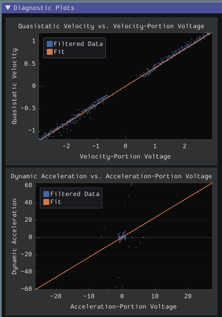
As our data look reasonably linear and our threshold seems to be set correctly, we may move on to the next step.
Note
Feedforward gains do not, in general, transfer across robots. Do not use the gains from this tutorial for your own robot.
We now record the feedforward gains calculated by the tool:
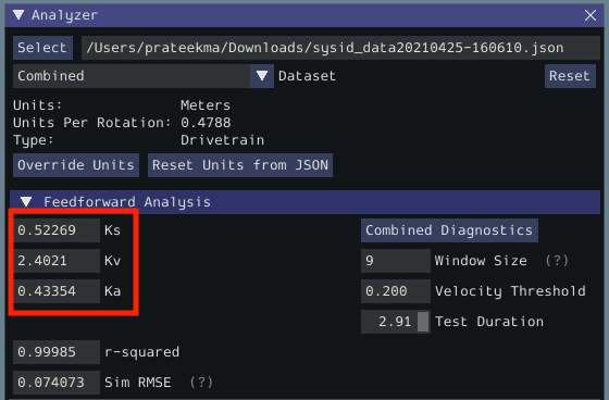
Since our wheel diameter was specified in meters, our feedforward gains are in the following units:
kS: VoltskV: Volts * Seconds / MeterskA: Volts * Seconds^2 / Meters
If you have specified your units correctly, your feedforward gains will likely be within an order of magnitude of the ones reported here (a possible exception exists for kA, which may be vanishingly small if your robot is light). If they are not, it is possible you specified one of your drive parameters incorrectly when generating your robot project. A good test for this is to calculate the “theoretical” value of kV, which is 12 volts divided by the theoretical free speed of your drivetrain (which is, in turn, the free speed of the motor times the wheel circumference divided by the gear reduction). This value should agree very closely with the kV measured by the tool - if it does not, you have likely made an error somewhere.
Note
Feedback gains do not, in general, transfer across robots. Do not use the gains from this tutorial for your own robot.
We now calculate the feedback gains for the PID control that we will use to follow the path. Trajectory following with WPILib’s RAMSETE controller uses velocity closed-loop control, so we first select Velocity mode in the characterization tool:
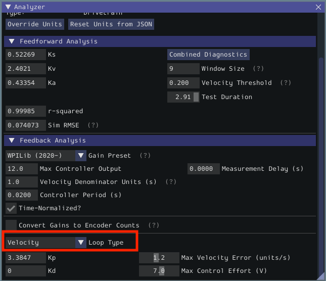
Since we will be using the WPILib PIDController for our velocity loop, we furthermore select the WPILib (2020-) option from the drop-down “presets” menu. This is very important, as the feedback gains will not be in the correct units if we do not select the correct preset:
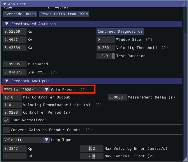
Finally, we calculate and record the feedback gains for our control loop. Since it is a velocity controller, only a P gain is required:
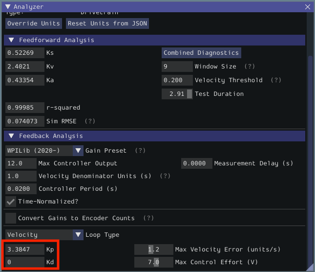
Assuming we have done everything correctly, our proportional gain will be in units of Volts * Seconds / Meters. Thus, our calculated gain means that, for each meter per second of velocity error, the controller will output an additional 3.38 volts.
Step 2: Entering the Calculated Constants
Note
In C++, it is important that the feedforward constants be entered as the correct unit type. For more information on C++ units, see The C++ Units Library.
Now that we have our characterization constants, it is time to place them in our code. The recommended place for this is the Constants file of the standard command-based project structure.
The relevant parts of the constants file from the RamseteCommand Example Project (Java, C++) can be seen below.
Feedforward/Feedback Gains
Firstly, we must enter the feedforward and feedback gains which we obtained from the characterization tool.
Note
Feedforward and feedback gains do not, in general, transfer across robots. Do not use the gains from this tutorial for your own robot.
44 // These are example values only - DO NOT USE THESE FOR YOUR OWN ROBOT!
45 // These characterization values MUST be determined either experimentally or theoretically
46 // for *your* robot's drive.
47 // The Robot Characterization Toolsuite provides a convenient tool for obtaining these
48 // values for your robot.
49 public static final double ksVolts = 0.22;
50 public static final double kvVoltSecondsPerMeter = 1.98;
51 public static final double kaVoltSecondsSquaredPerMeter = 0.2;
52
53 // Example value only - as above, this must be tuned for your drive!
54 public static final double kPDriveVel = 8.5;
46// These are example values only - DO NOT USE THESE FOR YOUR OWN ROBOT!
47// These characterization values MUST be determined either experimentally or
48// theoretically for *your* robot's drive. The Robot Characterization
49// Toolsuite provides a convenient tool for obtaining these values for your
50// robot.
51constexpr auto ks = 0.22_V;
52constexpr auto kv = 1.98 * 1_V * 1_s / 1_m;
53constexpr auto ka = 0.2 * 1_V * 1_s * 1_s / 1_m;
54
55// Example value only - as above, this must be tuned for your drive!
56constexpr double kPDriveVel = 8.5;
DifferentialDriveKinematics
Additionally, we must create an instance of the DifferentialDriveKinematics class, which allows us to use the trackwidth (i.e. horizontal distance between the wheels) of the robot to convert from chassis speeds to wheel speeds. As elsewhere, we keep our units in meters.
32 public static final double kTrackwidthMeters = 0.69;
33 public static final DifferentialDriveKinematics kDriveKinematics =
34 new DifferentialDriveKinematics(kTrackwidthMeters);
35constexpr auto kTrackwidth = 0.69_m;
36extern const frc::DifferentialDriveKinematics kDriveKinematics;
Max Trajectory Velocity/Acceleration
We must also decide on a nominal max acceleration and max velocity for the robot during path-following. The maximum velocity value should be set somewhat below the nominal free-speed of the robot. Due to the later use of the DifferentialDriveVoltageConstraint, the maximum acceleration value is not extremely crucial.
62 public static final double kMaxSpeedMetersPerSecond = 3;
63 public static final double kMaxAccelerationMetersPerSecondSquared = 3;
60constexpr auto kMaxSpeed = 3_mps;
61constexpr auto kMaxAcceleration = 3_mps_sq;
Ramsete Parameters
Finally, we must include a pair of parameters for the RAMSETE controller. The values shown below should work well for most robots, provided distances have been correctly measured in meters - for more information on tuning these values (if it is required), see Constructing the Ramsete Controller Object.
65 // Reasonable baseline values for a RAMSETE follower in units of meters and seconds
66 public static final double kRamseteB = 2;
67 public static final double kRamseteZeta = 0.7;
63// Reasonable baseline values for a RAMSETE follower in units of meters and
64// seconds
65constexpr double kRamseteB = 2;
66constexpr double kRamseteZeta = 0.7;
Step 3: Creating a Drive Subsystem
Now that our drive is characterized, it is time to start writing our robot code proper. As mentioned before, we will use the command-based framework for our robot code. Accordingly, our first step is to write a suitable drive subsystem class.
The full drive class from the RamseteCommand Example Project (Java, C++) can be seen below. The rest of the article will describe the steps involved in writing this class.
5package edu.wpi.first.wpilibj.examples.ramsetecommand.subsystems;
6
7import edu.wpi.first.math.geometry.Pose2d;
8import edu.wpi.first.math.kinematics.DifferentialDriveOdometry;
9import edu.wpi.first.math.kinematics.DifferentialDriveWheelSpeeds;
10import edu.wpi.first.wpilibj.ADXRS450_Gyro;
11import edu.wpi.first.wpilibj.Encoder;
12import edu.wpi.first.wpilibj.drive.DifferentialDrive;
13import edu.wpi.first.wpilibj.examples.ramsetecommand.Constants.DriveConstants;
14import edu.wpi.first.wpilibj.interfaces.Gyro;
15import edu.wpi.first.wpilibj.motorcontrol.MotorControllerGroup;
16import edu.wpi.first.wpilibj.motorcontrol.PWMSparkMax;
17import edu.wpi.first.wpilibj2.command.SubsystemBase;
18
19public class DriveSubsystem extends SubsystemBase {
20 // The motors on the left side of the drive.
21 private final MotorControllerGroup m_leftMotors =
22 new MotorControllerGroup(
23 new PWMSparkMax(DriveConstants.kLeftMotor1Port),
24 new PWMSparkMax(DriveConstants.kLeftMotor2Port));
25
26 // The motors on the right side of the drive.
27 private final MotorControllerGroup m_rightMotors =
28 new MotorControllerGroup(
29 new PWMSparkMax(DriveConstants.kRightMotor1Port),
30 new PWMSparkMax(DriveConstants.kRightMotor2Port));
31
32 // The robot's drive
33 private final DifferentialDrive m_drive = new DifferentialDrive(m_leftMotors, m_rightMotors);
34
35 // The left-side drive encoder
36 private final Encoder m_leftEncoder =
37 new Encoder(
38 DriveConstants.kLeftEncoderPorts[0],
39 DriveConstants.kLeftEncoderPorts[1],
40 DriveConstants.kLeftEncoderReversed);
41
42 // The right-side drive encoder
43 private final Encoder m_rightEncoder =
44 new Encoder(
45 DriveConstants.kRightEncoderPorts[0],
46 DriveConstants.kRightEncoderPorts[1],
47 DriveConstants.kRightEncoderReversed);
48
49 // The gyro sensor
50 private final Gyro m_gyro = new ADXRS450_Gyro();
51
52 // Odometry class for tracking robot pose
53 private final DifferentialDriveOdometry m_odometry;
54
55 /** Creates a new DriveSubsystem. */
56 public DriveSubsystem() {
57 // We need to invert one side of the drivetrain so that positive voltages
58 // result in both sides moving forward. Depending on how your robot's
59 // gearbox is constructed, you might have to invert the left side instead.
60 m_rightMotors.setInverted(true);
61
62 // Sets the distance per pulse for the encoders
63 m_leftEncoder.setDistancePerPulse(DriveConstants.kEncoderDistancePerPulse);
64 m_rightEncoder.setDistancePerPulse(DriveConstants.kEncoderDistancePerPulse);
65
66 resetEncoders();
67 m_odometry = new DifferentialDriveOdometry(m_gyro.getRotation2d());
68 }
69
70 @Override
71 public void periodic() {
72 // Update the odometry in the periodic block
73 m_odometry.update(
74 m_gyro.getRotation2d(), m_leftEncoder.getDistance(), m_rightEncoder.getDistance());
75 }
76
77 /**
78 * Returns the currently-estimated pose of the robot.
79 *
80 * @return The pose.
81 */
82 public Pose2d getPose() {
83 return m_odometry.getPoseMeters();
84 }
85
86 /**
87 * Returns the current wheel speeds of the robot.
88 *
89 * @return The current wheel speeds.
90 */
91 public DifferentialDriveWheelSpeeds getWheelSpeeds() {
92 return new DifferentialDriveWheelSpeeds(m_leftEncoder.getRate(), m_rightEncoder.getRate());
93 }
94
95 /**
96 * Resets the odometry to the specified pose.
97 *
98 * @param pose The pose to which to set the odometry.
99 */
100 public void resetOdometry(Pose2d pose) {
101 resetEncoders();
102 m_odometry.resetPosition(pose, m_gyro.getRotation2d());
103 }
104
105 /**
106 * Drives the robot using arcade controls.
107 *
108 * @param fwd the commanded forward movement
109 * @param rot the commanded rotation
110 */
111 public void arcadeDrive(double fwd, double rot) {
112 m_drive.arcadeDrive(fwd, rot);
113 }
114
115 /**
116 * Controls the left and right sides of the drive directly with voltages.
117 *
118 * @param leftVolts the commanded left output
119 * @param rightVolts the commanded right output
120 */
121 public void tankDriveVolts(double leftVolts, double rightVolts) {
122 m_leftMotors.setVoltage(leftVolts);
123 m_rightMotors.setVoltage(rightVolts);
124 m_drive.feed();
125 }
126
127 /** Resets the drive encoders to currently read a position of 0. */
128 public void resetEncoders() {
129 m_leftEncoder.reset();
130 m_rightEncoder.reset();
131 }
132
133 /**
134 * Gets the average distance of the two encoders.
135 *
136 * @return the average of the two encoder readings
137 */
138 public double getAverageEncoderDistance() {
139 return (m_leftEncoder.getDistance() + m_rightEncoder.getDistance()) / 2.0;
140 }
141
142 /**
143 * Gets the left drive encoder.
144 *
145 * @return the left drive encoder
146 */
147 public Encoder getLeftEncoder() {
148 return m_leftEncoder;
149 }
150
151 /**
152 * Gets the right drive encoder.
153 *
154 * @return the right drive encoder
155 */
156 public Encoder getRightEncoder() {
157 return m_rightEncoder;
158 }
159
160 /**
161 * Sets the max output of the drive. Useful for scaling the drive to drive more slowly.
162 *
163 * @param maxOutput the maximum output to which the drive will be constrained
164 */
165 public void setMaxOutput(double maxOutput) {
166 m_drive.setMaxOutput(maxOutput);
167 }
168
169 /** Zeroes the heading of the robot. */
170 public void zeroHeading() {
171 m_gyro.reset();
172 }
173
174 /**
175 * Returns the heading of the robot.
176 *
177 * @return the robot's heading in degrees, from -180 to 180
178 */
179 public double getHeading() {
180 return m_gyro.getRotation2d().getDegrees();
181 }
182
183 /**
184 * Returns the turn rate of the robot.
185 *
186 * @return The turn rate of the robot, in degrees per second
187 */
188 public double getTurnRate() {
189 return -m_gyro.getRate();
190 }
191}
5#pragma once
6
7#include <frc/ADXRS450_Gyro.h>
8#include <frc/Encoder.h>
9#include <frc/drive/DifferentialDrive.h>
10#include <frc/geometry/Pose2d.h>
11#include <frc/kinematics/DifferentialDriveOdometry.h>
12#include <frc/motorcontrol/MotorControllerGroup.h>
13#include <frc/motorcontrol/PWMSparkMax.h>
14#include <frc2/command/SubsystemBase.h>
15#include <units/voltage.h>
16
17#include "Constants.h"
18
19class DriveSubsystem : public frc2::SubsystemBase {
20 public:
21 DriveSubsystem();
22
23 /**
24 * Will be called periodically whenever the CommandScheduler runs.
25 */
26 void Periodic() override;
27
28 // Subsystem methods go here.
29
30 /**
31 * Drives the robot using arcade controls.
32 *
33 * @param fwd the commanded forward movement
34 * @param rot the commanded rotation
35 */
36 void ArcadeDrive(double fwd, double rot);
37
38 /**
39 * Controls each side of the drive directly with a voltage.
40 *
41 * @param left the commanded left output
42 * @param right the commanded right output
43 */
44 void TankDriveVolts(units::volt_t left, units::volt_t right);
45
46 /**
47 * Resets the drive encoders to currently read a position of 0.
48 */
49 void ResetEncoders();
50
51 /**
52 * Gets the average distance of the TWO encoders.
53 *
54 * @return the average of the TWO encoder readings
55 */
56 double GetAverageEncoderDistance();
57
58 /**
59 * Gets the left drive encoder.
60 *
61 * @return the left drive encoder
62 */
63 frc::Encoder& GetLeftEncoder();
64
65 /**
66 * Gets the right drive encoder.
67 *
68 * @return the right drive encoder
69 */
70 frc::Encoder& GetRightEncoder();
71
72 /**
73 * Sets the max output of the drive. Useful for scaling the drive to drive
74 * more slowly.
75 *
76 * @param maxOutput the maximum output to which the drive will be constrained
77 */
78 void SetMaxOutput(double maxOutput);
79
80 /**
81 * Returns the heading of the robot.
82 *
83 * @return the robot's heading in degrees, from -180 to 180
84 */
85 units::degree_t GetHeading() const;
86
87 /**
88 * Returns the turn rate of the robot.
89 *
90 * @return The turn rate of the robot, in degrees per second
91 */
92 double GetTurnRate();
93
94 /**
95 * Returns the currently-estimated pose of the robot.
96 *
97 * @return The pose.
98 */
99 frc::Pose2d GetPose();
100
101 /**
102 * Returns the current wheel speeds of the robot.
103 *
104 * @return The current wheel speeds.
105 */
106 frc::DifferentialDriveWheelSpeeds GetWheelSpeeds();
107
108 /**
109 * Resets the odometry to the specified pose.
110 *
111 * @param pose The pose to which to set the odometry.
112 */
113 void ResetOdometry(frc::Pose2d pose);
114
115 private:
116 // Components (e.g. motor controllers and sensors) should generally be
117 // declared private and exposed only through public methods.
118
119 // The motor controllers
120 frc::PWMSparkMax m_left1;
121 frc::PWMSparkMax m_left2;
122 frc::PWMSparkMax m_right1;
123 frc::PWMSparkMax m_right2;
124
125 // The motors on the left side of the drive
126 frc::MotorControllerGroup m_leftMotors{m_left1, m_left2};
127
128 // The motors on the right side of the drive
129 frc::MotorControllerGroup m_rightMotors{m_right1, m_right2};
130
131 // The robot's drive
132 frc::DifferentialDrive m_drive{m_leftMotors, m_rightMotors};
133
134 // The left-side drive encoder
135 frc::Encoder m_leftEncoder;
136
137 // The right-side drive encoder
138 frc::Encoder m_rightEncoder;
139
140 // The gyro sensor
141 frc::ADXRS450_Gyro m_gyro;
142
143 // Odometry class for tracking robot pose
144 frc::DifferentialDriveOdometry m_odometry;
145};
5#include "subsystems/DriveSubsystem.h"
6
7#include <frc/geometry/Rotation2d.h>
8#include <frc/kinematics/DifferentialDriveWheelSpeeds.h>
9
10using namespace DriveConstants;
11
12DriveSubsystem::DriveSubsystem()
13 : m_left1{kLeftMotor1Port},
14 m_left2{kLeftMotor2Port},
15 m_right1{kRightMotor1Port},
16 m_right2{kRightMotor2Port},
17 m_leftEncoder{kLeftEncoderPorts[0], kLeftEncoderPorts[1]},
18 m_rightEncoder{kRightEncoderPorts[0], kRightEncoderPorts[1]},
19 m_odometry{m_gyro.GetRotation2d()} {
20 // We need to invert one side of the drivetrain so that positive voltages
21 // result in both sides moving forward. Depending on how your robot's
22 // gearbox is constructed, you might have to invert the left side instead.
23 m_rightMotors.SetInverted(true);
24
25 // Set the distance per pulse for the encoders
26 m_leftEncoder.SetDistancePerPulse(kEncoderDistancePerPulse);
27 m_rightEncoder.SetDistancePerPulse(kEncoderDistancePerPulse);
28
29 ResetEncoders();
30}
31
32void DriveSubsystem::Periodic() {
33 // Implementation of subsystem periodic method goes here.
34 m_odometry.Update(m_gyro.GetRotation2d(),
35 units::meter_t(m_leftEncoder.GetDistance()),
36 units::meter_t(m_rightEncoder.GetDistance()));
37}
38
39void DriveSubsystem::ArcadeDrive(double fwd, double rot) {
40 m_drive.ArcadeDrive(fwd, rot);
41}
42
43void DriveSubsystem::TankDriveVolts(units::volt_t left, units::volt_t right) {
44 m_leftMotors.SetVoltage(left);
45 m_rightMotors.SetVoltage(right);
46 m_drive.Feed();
47}
48
49void DriveSubsystem::ResetEncoders() {
50 m_leftEncoder.Reset();
51 m_rightEncoder.Reset();
52}
53
54double DriveSubsystem::GetAverageEncoderDistance() {
55 return (m_leftEncoder.GetDistance() + m_rightEncoder.GetDistance()) / 2.0;
56}
57
58frc::Encoder& DriveSubsystem::GetLeftEncoder() {
59 return m_leftEncoder;
60}
61
62frc::Encoder& DriveSubsystem::GetRightEncoder() {
63 return m_rightEncoder;
64}
65
66void DriveSubsystem::SetMaxOutput(double maxOutput) {
67 m_drive.SetMaxOutput(maxOutput);
68}
69
70units::degree_t DriveSubsystem::GetHeading() const {
71 return m_gyro.GetRotation2d().Degrees();
72}
73
74double DriveSubsystem::GetTurnRate() {
75 return -m_gyro.GetRate();
76}
77
78frc::Pose2d DriveSubsystem::GetPose() {
79 return m_odometry.GetPose();
80}
81
82frc::DifferentialDriveWheelSpeeds DriveSubsystem::GetWheelSpeeds() {
83 return {units::meters_per_second_t(m_leftEncoder.GetRate()),
84 units::meters_per_second_t(m_rightEncoder.GetRate())};
85}
86
87void DriveSubsystem::ResetOdometry(frc::Pose2d pose) {
88 ResetEncoders();
89 m_odometry.ResetPosition(pose, m_gyro.GetRotation2d());
90}
Configuring the Drive Encoders
The drive encoders measure the rotation of the wheels on each side of the drive. To properly configure the encoders, we need to specify two things: the ports the encoders are plugged into, and the distance per encoder pulse. Then, we need to write methods allowing access to the encoder values from code that uses the subsystem.
The encoder ports are specified in the encoder’s constructor, like so:
35 // The left-side drive encoder
36 private final Encoder m_leftEncoder =
37 new Encoder(
38 DriveConstants.kLeftEncoderPorts[0],
39 DriveConstants.kLeftEncoderPorts[1],
40 DriveConstants.kLeftEncoderReversed);
41
42 // The right-side drive encoder
43 private final Encoder m_rightEncoder =
44 new Encoder(
45 DriveConstants.kRightEncoderPorts[0],
46 DriveConstants.kRightEncoderPorts[1],
47 DriveConstants.kRightEncoderReversed);
17 m_leftEncoder{kLeftEncoderPorts[0], kLeftEncoderPorts[1]},
18 m_rightEncoder{kRightEncoderPorts[0], kRightEncoderPorts[1]},
The distance per pulse is specified by calling the encoder’s setDistancePerPulse method. Note that for the WPILib Encoder class, “pulse” refers to a full encoder cycle (i.e. four edges), and thus will be 1/4 the value that was specified in the FRC-Characterization config. Remember, as well, that the distance should be measured in meters!
63 m_leftEncoder.setDistancePerPulse(DriveConstants.kEncoderDistancePerPulse);
64 m_rightEncoder.setDistancePerPulse(DriveConstants.kEncoderDistancePerPulse);
26 m_leftEncoder.SetDistancePerPulse(kEncoderDistancePerPulse);
27 m_rightEncoder.SetDistancePerPulse(kEncoderDistancePerPulse);
To access the values measured by the encoders, we include the following method:
Important
The returned velocities must be in meters! Because we configured the distance per pulse on the encoders above, calling getRate() will automatically apply the conversion factor from encoder units to meters. If you are not using WPILib’s Encoder class, you must perform this conversion either through the respective vendor’s API or by manually multiplying by a conversion factor.
86 /**
87 * Returns the current wheel speeds of the robot.
88 *
89 * @return The current wheel speeds.
90 */
91 public DifferentialDriveWheelSpeeds getWheelSpeeds() {
92 return new DifferentialDriveWheelSpeeds(m_leftEncoder.getRate(), m_rightEncoder.getRate());
93 }
82frc::DifferentialDriveWheelSpeeds DriveSubsystem::GetWheelSpeeds() {
83 return {units::meters_per_second_t(m_leftEncoder.GetRate()),
84 units::meters_per_second_t(m_rightEncoder.GetRate())};
85}
We wrap the measured encoder values in a DifferentialDriveWheelSpeeds object for easier integration with the RamseteCommand class later on.
Configuring the Gyroscope
The gyroscope measures the rate of change of the robot’s heading (which can then be integrated to provide a measurement of the robot’s heading relative to when it first turned on). In our example, we use the Analog Devices ADXRS450 FRC Gyro Board, which has been included in the kit of parts for several years:
50 private final Gyro m_gyro = new ADXRS450_Gyro();
140 // The gyro sensor
141 frc::ADXRS450_Gyro m_gyro;
To access the current heading measured by the gyroscope, we include the following method:
174 /**
175 * Returns the heading of the robot.
176 *
177 * @return the robot's heading in degrees, from -180 to 180
178 */
179 public double getHeading() {
180 return m_gyro.getRotation2d().getDegrees();
181 }
70units::degree_t DriveSubsystem::GetHeading() const {
71 return m_gyro.GetRotation2d().Degrees();
72}
Configuring the Odometry
Now that we have our encoders and gyroscope configured, it is time to set up our drive subsystem to automatically compute its position from the encoder and gyroscope readings.
First, we create a member instance of the DifferentialDriveOdometry class:
53 // Odometry class for tracking robot pose
54 private final DifferentialDriveOdometry m_odometry;
143 // Odometry class for tracking robot pose
144 frc::DifferentialDriveOdometry m_odometry;
The odometry class must be regularly updated to incorporate new readings from the encoder and gyroscope. We accomplish this inside the subsystem’s periodic method, which is automatically called once per main loop iteration:
70 @Override
71 public void periodic() {
72 // Update the odometry in the periodic block
73 m_odometry.update(
74 m_gyro.getRotation2d(), m_leftEncoder.getDistance(), m_rightEncoder.getDistance());
75 }
32void DriveSubsystem::Periodic() {
33 // Implementation of subsystem periodic method goes here.
34 m_odometry.Update(m_gyro.GetRotation2d(),
35 units::meter_t(m_leftEncoder.GetDistance()),
36 units::meter_t(m_rightEncoder.GetDistance()));
37}
To access the robot’s current computed pose, we include the following method:
74 /**
75 * Returns the currently-estimated pose of the robot.
76 *
77 * @return The pose.
78 */
79 public Pose2d getPose() {
80 return m_odometry.getPoseMeters();
81 }
78frc::Pose2d DriveSubsystem::GetPose() {
79 return m_odometry.GetPose();
80}
Voltage-Based Drive Method
Finally, we must include one additional method - a method that allows us to set the voltage to each side of the drive using the setVoltage() method of the MotorController interface. The default WPILib drive class does not include this functionality, so we must write it ourselves:
125 /**
126 * Controls the left and right sides of the drive directly with voltages.
127 *
128 * @param leftVolts the commanded left output
129 * @param rightVolts the commanded right output
130 */
131 public void tankDriveVolts(double leftVolts, double rightVolts) {
132 m_leftMotors.setVoltage(leftVolts);
133 m_rightMotors.setVoltage(rightVolts);
134 m_drive.feed();
135 }
43void DriveSubsystem::TankDriveVolts(units::volt_t left, units::volt_t right) {
44 m_leftMotors.SetVoltage(left);
45 m_rightMotors.SetVoltage(right);
46 m_drive.Feed();
47}
It is very important to use the setVoltage() method rather than the ordinary set() method, as this will automatically compensate for battery “voltage sag” during operation. Since our feedforward voltages are physically-meaningful (as they are based on measured characterization data), this is essential to ensuring their accuracy.
Step 4: Creating and Following a Trajectory
With our drive subsystem written, it is now time to generate a trajectory and write an autonomous command to follow it.
As per the standard command-based project structure, we will do this in the getAutonomousCommand method of the RobotContainer class. The full method from the RamseteCommand Example Project (Java, C++) can be seen below. The rest of the article will break down the different parts of the method in more detail.
75 /**
76 * Use this to pass the autonomous command to the main {@link Robot} class.
77 *
78 * @return the command to run in autonomous
79 */
80 public Command getAutonomousCommand() {
81
82 // Create a voltage constraint to ensure we don't accelerate too fast
83 var autoVoltageConstraint =
84 new DifferentialDriveVoltageConstraint(
85 new SimpleMotorFeedforward(
86 DriveConstants.ksVolts,
87 DriveConstants.kvVoltSecondsPerMeter,
88 DriveConstants.kaVoltSecondsSquaredPerMeter),
89 DriveConstants.kDriveKinematics,
90 10);
91
92 // Create config for trajectory
93 TrajectoryConfig config =
94 new TrajectoryConfig(
95 AutoConstants.kMaxSpeedMetersPerSecond,
96 AutoConstants.kMaxAccelerationMetersPerSecondSquared)
97 // Add kinematics to ensure max speed is actually obeyed
98 .setKinematics(DriveConstants.kDriveKinematics)
99 // Apply the voltage constraint
100 .addConstraint(autoVoltageConstraint);
101
102 // An example trajectory to follow. All units in meters.
103 Trajectory exampleTrajectory =
104 TrajectoryGenerator.generateTrajectory(
105 // Start at the origin facing the +X direction
106 new Pose2d(0, 0, new Rotation2d(0)),
107 // Pass through these two interior waypoints, making an 's' curve path
108 List.of(new Translation2d(1, 1), new Translation2d(2, -1)),
109 // End 3 meters straight ahead of where we started, facing forward
110 new Pose2d(3, 0, new Rotation2d(0)),
111 // Pass config
112 config);
113
114 RamseteCommand ramseteCommand =
115 new RamseteCommand(
116 exampleTrajectory,
117 m_robotDrive::getPose,
118 new RamseteController(AutoConstants.kRamseteB, AutoConstants.kRamseteZeta),
119 new SimpleMotorFeedforward(
120 DriveConstants.ksVolts,
121 DriveConstants.kvVoltSecondsPerMeter,
122 DriveConstants.kaVoltSecondsSquaredPerMeter),
123 DriveConstants.kDriveKinematics,
124 m_robotDrive::getWheelSpeeds,
125 new PIDController(DriveConstants.kPDriveVel, 0, 0),
126 new PIDController(DriveConstants.kPDriveVel, 0, 0),
127 // RamseteCommand passes volts to the callback
128 m_robotDrive::tankDriveVolts,
129 m_robotDrive);
130
131 // Reset odometry to the starting pose of the trajectory.
132 m_robotDrive.resetOdometry(exampleTrajectory.getInitialPose());
133
134 // Run path following command, then stop at the end.
135 return ramseteCommand.andThen(() -> m_robotDrive.tankDriveVolts(0, 0));
136 }
137}
47frc2::Command* RobotContainer::GetAutonomousCommand() {
48 // Create a voltage constraint to ensure we don't accelerate too fast
49 frc::DifferentialDriveVoltageConstraint autoVoltageConstraint(
50 frc::SimpleMotorFeedforward<units::meters>(
51 DriveConstants::ks, DriveConstants::kv, DriveConstants::ka),
52 DriveConstants::kDriveKinematics, 10_V);
53
54 // Set up config for trajectory
55 frc::TrajectoryConfig config(AutoConstants::kMaxSpeed,
56 AutoConstants::kMaxAcceleration);
57 // Add kinematics to ensure max speed is actually obeyed
58 config.SetKinematics(DriveConstants::kDriveKinematics);
59 // Apply the voltage constraint
60 config.AddConstraint(autoVoltageConstraint);
61
62 // An example trajectory to follow. All units in meters.
63 auto exampleTrajectory = frc::TrajectoryGenerator::GenerateTrajectory(
64 // Start at the origin facing the +X direction
65 frc::Pose2d(0_m, 0_m, frc::Rotation2d(0_deg)),
66 // Pass through these two interior waypoints, making an 's' curve path
67 {frc::Translation2d(1_m, 1_m), frc::Translation2d(2_m, -1_m)},
68 // End 3 meters straight ahead of where we started, facing forward
69 frc::Pose2d(3_m, 0_m, frc::Rotation2d(0_deg)),
70 // Pass the config
71 config);
72
73 frc2::RamseteCommand ramseteCommand(
74 exampleTrajectory, [this]() { return m_drive.GetPose(); },
75 frc::RamseteController(AutoConstants::kRamseteB,
76 AutoConstants::kRamseteZeta),
77 frc::SimpleMotorFeedforward<units::meters>(
78 DriveConstants::ks, DriveConstants::kv, DriveConstants::ka),
79 DriveConstants::kDriveKinematics,
80 [this] { return m_drive.GetWheelSpeeds(); },
81 frc2::PIDController(DriveConstants::kPDriveVel, 0, 0),
82 frc2::PIDController(DriveConstants::kPDriveVel, 0, 0),
83 [this](auto left, auto right) { m_drive.TankDriveVolts(left, right); },
84 {&m_drive});
85
86 // Reset odometry to the starting pose of the trajectory.
87 m_drive.ResetOdometry(exampleTrajectory.InitialPose());
88
89 // no auto
90 return new frc2::SequentialCommandGroup(
91 std::move(ramseteCommand),
92 frc2::InstantCommand([this] { m_drive.TankDriveVolts(0_V, 0_V); }, {}));
Configuring the Trajectory Constraints
First, we must set some configuration parameters for the trajectory which will ensure that the generated trajectory is followable.
The first piece of configuration we will need is a voltage constraint. This will ensure that the generated trajectory never commands the robot to go faster than it is capable of achieving with the given voltage supply:
89 // Create a voltage constraint to ensure we don't accelerate too fast
90 var autoVoltageConstraint =
91 new DifferentialDriveVoltageConstraint(
92 new SimpleMotorFeedforward(DriveConstants.ksVolts,
93 DriveConstants.kvVoltSecondsPerMeter,
94 DriveConstants.kaVoltSecondsSquaredPerMeter),
95 DriveConstants.kDriveKinematics,
96 10);
48 // Create a voltage constraint to ensure we don't accelerate too fast
49 frc::DifferentialDriveVoltageConstraint autoVoltageConstraint(
50 frc::SimpleMotorFeedforward<units::meters>(
51 DriveConstants::ks, DriveConstants::kv, DriveConstants::ka),
52 DriveConstants::kDriveKinematics, 10_V);
Notice that we set the maximum voltage to 10V, rather than the nominal battery voltage of 12V. This gives us some “headroom” to deal with “voltage sag” during operation.
Now that we have our voltage constraint, we can create our TrajectoryConfig instance, which wraps together all of our path constraints:
98 // Create config for trajectory
99 TrajectoryConfig config =
100 new TrajectoryConfig(AutoConstants.kMaxSpeedMetersPerSecond,
101 AutoConstants.kMaxAccelerationMetersPerSecondSquared)
102 // Add kinematics to ensure max speed is actually obeyed
103 .setKinematics(DriveConstants.kDriveKinematics)
104 // Apply the voltage constraint
105 .addConstraint(autoVoltageConstraint);
54 // Set up config for trajectory
55 frc::TrajectoryConfig config(AutoConstants::kMaxSpeed,
56 AutoConstants::kMaxAcceleration);
57 // Add kinematics to ensure max speed is actually obeyed
58 config.SetKinematics(DriveConstants::kDriveKinematics);
59 // Apply the voltage constraint
60 config.AddConstraint(autoVoltageConstraint);
Generating the Trajectory
With our trajectory configuration in hand, we are now ready to generate our trajectory. For this example, we will be generating a “clamped cubic” trajectory - this means we will specify full robot poses at the endpoints, and positions only for interior waypoints (also known as “knot points”). As elsewhere, all distances are in meters.
108 Trajectory exampleTrajectory = TrajectoryGenerator.generateTrajectory(
109 // Start at the origin facing the +X direction
110 new Pose2d(0, 0, new Rotation2d(0)),
111 // Pass through these two interior waypoints, making an 's' curve path
112 List.of(
113 new Translation2d(1, 1),
114 new Translation2d(2, -1)
115 ),
116 // End 3 meters straight ahead of where we started, facing forward
117 new Pose2d(3, 0, new Rotation2d(0)),
118 // Pass config
119 config
120 );
62 // An example trajectory to follow. All units in meters.
63 auto exampleTrajectory = frc::TrajectoryGenerator::GenerateTrajectory(
64 // Start at the origin facing the +X direction
65 frc::Pose2d(0_m, 0_m, frc::Rotation2d(0_deg)),
66 // Pass through these two interior waypoints, making an 's' curve path
67 {frc::Translation2d(1_m, 1_m), frc::Translation2d(2_m, -1_m)},
68 // End 3 meters straight ahead of where we started, facing forward
69 frc::Pose2d(3_m, 0_m, frc::Rotation2d(0_deg)),
70 // Pass the config
71 config);
Note
Instead of generating the trajectory on the roboRIO as outlined above, one can also import a PathWeaver JSON.
Creating the RamseteCommand
We will first reset our robot’s pose to the starting pose of the trajectory. This ensures that the robot’s location on the coordinate system and the trajectory’s starting position are the same.
137 // Reset odometry to the starting pose of the trajectory.
138 m_robotDrive.resetOdometry(exampleTrajectory.getInitialPose());
86 // Reset odometry to the starting pose of the trajectory.
87 m_drive.ResetOdometry(exampleTrajectory.InitialPose());
It is very important that the initial robot pose match the first pose in the trajectory. For the purposes of our example, the robot will be reliably starting at a position of (0,0) with a heading of 0. In actual use, however, it is probably not desirable to base your coordinate system on the robot position, and so the starting position for both the robot and the trajectory should be set to some other value. If you wish to use a trajectory that has been defined in robot-centric coordinates in such a situation, you can transform it to be relative to the robot’s current pose using the transformBy method (Java, C++). For more information about transforming trajectories, see Transforming Trajectories.
Now that we have a trajectory, we can create a command that, when executed, will follow that trajectory. To do this, we use the RamseteCommand class (Java, C++)
122 RamseteCommand ramseteCommand = new RamseteCommand(
123 exampleTrajectory,
124 m_robotDrive::getPose,
125 new RamseteController(AutoConstants.kRamseteB, AutoConstants.kRamseteZeta),
126 new SimpleMotorFeedforward(DriveConstants.ksVolts,
127 DriveConstants.kvVoltSecondsPerMeter,
128 DriveConstants.kaVoltSecondsSquaredPerMeter),
129 DriveConstants.kDriveKinematics,
130 m_robotDrive::getWheelSpeeds,
131 new PIDController(DriveConstants.kPDriveVel, 0, 0),
132 new PIDController(DriveConstants.kPDriveVel, 0, 0),
133 // RamseteCommand passes volts to the callback
134 m_robotDrive::tankDriveVolts,
135 m_robotDrive
136 );
73 frc2::RamseteCommand ramseteCommand(
74 exampleTrajectory, [this]() { return m_drive.GetPose(); },
75 frc::RamseteController(AutoConstants::kRamseteB,
76 AutoConstants::kRamseteZeta),
77 frc::SimpleMotorFeedforward<units::meters>(
78 DriveConstants::ks, DriveConstants::kv, DriveConstants::ka),
79 DriveConstants::kDriveKinematics,
80 [this] { return m_drive.GetWheelSpeeds(); },
81 frc2::PIDController(DriveConstants::kPDriveVel, 0, 0),
82 frc2::PIDController(DriveConstants::kPDriveVel, 0, 0),
83 [this](auto left, auto right) { m_drive.TankDriveVolts(left, right); },
84 {&m_drive});
This declaration is fairly substantial, so we’ll go through it argument-by-argument:
The trajectory: This is the trajectory to be followed; accordingly, we pass the command the trajectory we just constructed in our earlier steps.
The pose supplier: This is a method reference (or lambda) to the drive subsystem method that returns the pose. The RAMSETE controller needs the current pose measurement to determine the required wheel outputs.
The RAMSETE controller: This is the
RamseteControllerobject (Java, C++) that will perform the path-following computation that translates the current measured pose and trajectory state into a chassis speed setpoint.The drive feedforward: This is a
SimpleMotorFeedforwardobject (Java, C++) that will automatically perform the correct feedforward calculation with the feedforward gains (kS,kV, andkA) that we obtained from the drive characterization tool.The drive kinematics: This is the
DifferentialDriveKinematicsobject (Java, C++) that we constructed earlier in our constants file, and will be used to convert chassis speeds to wheel speeds.The wheel speed supplier: This is a method reference (or lambda) to the drive subsystem method that returns the wheel speeds
The left-side PIDController: This is the
PIDControllerobject (Java, C++) that will track the left-side wheel speed setpoint, using the P gain that we obtained from the drive characterization tool.The right-side PIDController: This is the
PIDControllerobject (Java, C++) that will track the right-side wheel speed setpoint, using the P gain that we obtained from the drive characterization tool.The output consumer: This is a method reference (or lambda) to the drive subsystem method that passes the voltage outputs to the drive motors.
The robot drive: This is the drive subsystem itself, included to ensure the command does not operate on the drive at the same time as any other command that uses the drive.
Finally, note that we append a final “stop” command in sequence after the path-following command, to ensure that the robot stops moving at the end of the trajectory.
Video
If all has gone well, your robot’s autonomous routine should look something like this:
PathWeaver
Introduction to PathWeaver
Autonomous is an important section of the match; it is exciting when robots do impressive things in autonomous. In order to score, the robot usually need to go somewhere. The faster the robot arrives at that location, the sooner it can score points! The traditional method for autonomous is driving in a straight line, turning to a certain angle, and driving in a straight line again. This approach works fine, but the robot spends a non-negligible amount of time stopping and starting again after each straight line and turn.
A more advanced approach to autonomous is called “path planning”. Instead of driving in a straight line and turning once the line is complete, the robot continuously moves, driving with a curve-like motion. This can reduce turning stoppage time.
WPILib contains a trajectory generation suite that can be used by teams to generate and follow trajectories. This series of articles will go over how to generate and visualize trajectories using PathWeaver. For a comprehensive tutorial on following trajectories, please visit the end-to-end trajectory tutorial.
Note
Trajectory following code is required to use PathWeaver. We recommend that you start with Trajectory following and get that working with simple paths. From there you can continue on to testing more complicated paths generated by PathWeaver.
Creating a Pathweaver Project
PathWeaver is the tool used to draw the paths for a robot to follow. The paths for a single program are stored in a PathWeaver project.
Starting PathWeaver
PathWeaver is started by clicking on the ellipsis icon in the top right of the corner of the Visual Studio Code interface. You must select a source file from the WPILib project to see the icon. Then click on “Start tool” and then click on “PathWeaver” as shown below.
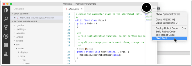
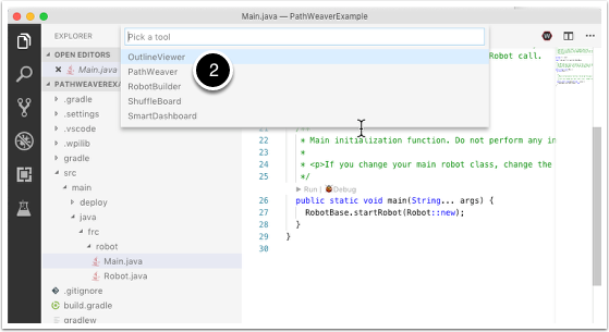
Creating the Project
To create a PathWeaver project, click on “Create project” and then fill out the project creation form. Notice that hovering over any of the fields in the form will display more information about what is required.
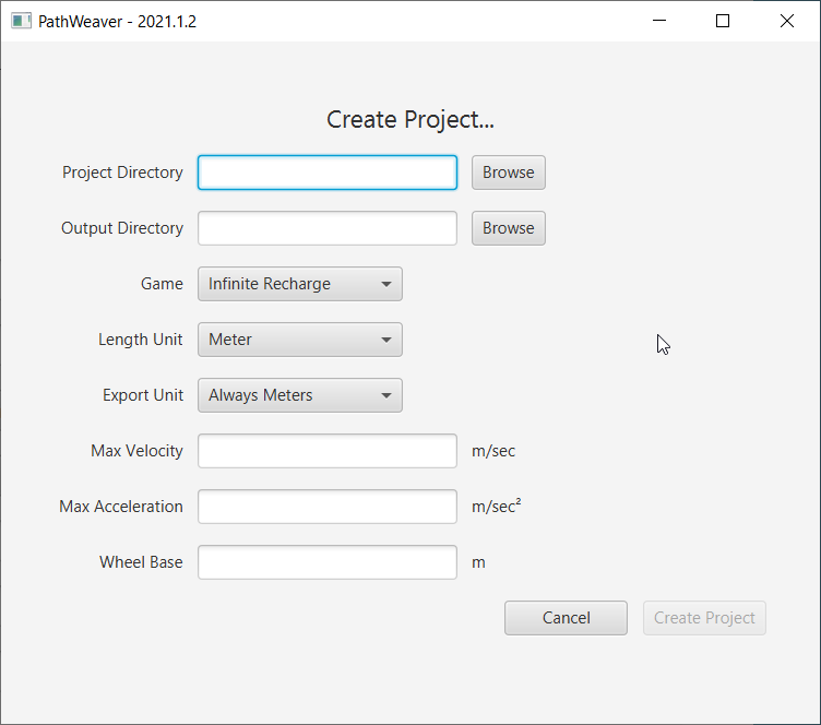
Project Directory: This is normally the top level project directory that contains the build.gradle and src files for your robot program. Choosing this directory is the expected way to use PathWeaver and will cause it to locate all the output files in the correct directories for automatic path deployment to your robot.
Output directory: The directory where the paths are stored for deployment to your robot. If you specified the top level project folder of our robot project in the previous step (as recommended) filling in the output directory is optional.
Game: The game (which FRC® game is being used) will cause the correct field image overlay to be used. You can also create your own field images and the procedure will be described later in this series.
Length Unit: The units to be used in describing your robot and for the field measurements when visualizing trajectories using PathWeaver.
Export Unit: The units to be used when exporting the paths and waypoints. If you are planning to use WPILib Trajectories, then you should choose Always Meters. Choosing Same as Project will export in the same units as Length Unit above.
Max Velocity: The max speed of the robot for trajectory tracking. This does not need to be the maximum attainable speed of the robot, but just the max speed that you want to run trajectories at.
Max Acceleration: The max acceleration of the robot for trajectory tracking. This does not need to be the maximum attainable acceleration of the robot, but just the max acceleration that you want to run trajectories at.
Wheel Base: The distance between the left and right wheels of your robot. This is used to ensure that no wheel on a differential drive will go over the specified max velocity around turns.
PathWeaver User Interface
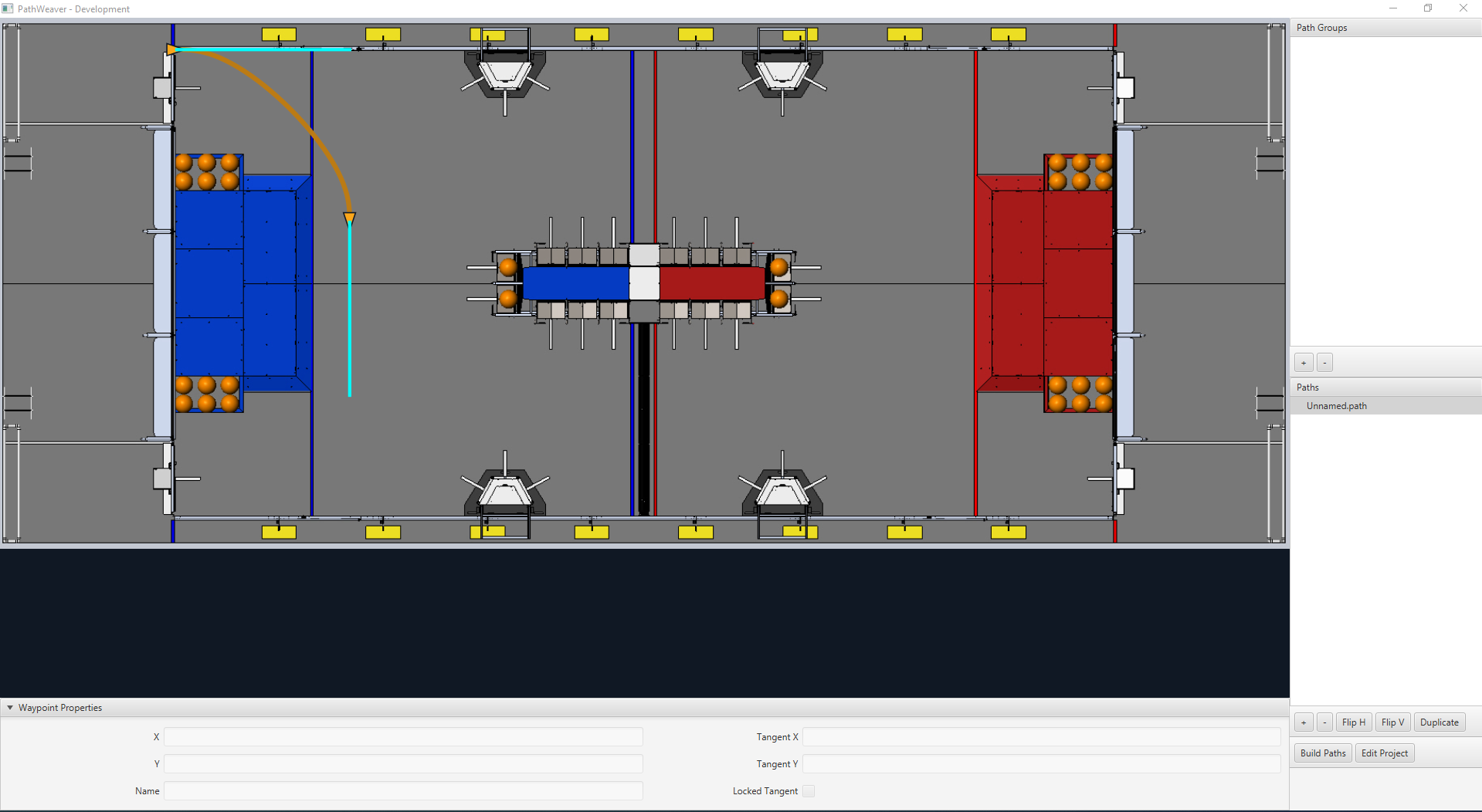
The PathWeaver user interface consists of the following:
The field area in the top left corner, which takes up most of the PathWeaver window. Trajectories are drawn on this part of the program.
The properties of the currently selected waypoint are displayed in the bottom pane. These properties include the X and Y, along with the tangents at each point.
A group of paths (or an “autonomous” mode) is displayed on the upper right side of the window. This is a convenient way of seeing all of the trajectories in a single auto mode.
The individual paths that a robot might follow are displayed in the lower right side of the window.
The “Build Paths” button will export the trajectories in a JSON format. These JSON files can be used from the robot code to follow the trajectory.
The “Edit Project” button allows you to edit the project properties.
Visualizing PathWeaver Trajectories
PathWeaver’s primary feature is to visualize trajectories. The following images depict a smooth trajectory that represents a trajectory that a robot might take during the autonomous period. Paths can have any number of waypoints that can allow more complex driving to be described. In this case there are 3 waypoints (including the start and stop) depicted with the triangle icons. Each waypoint consists of a X, Y position on the field as well as a robot heading described as the X and Y tangent lines.
Creating the Initial Trajectory
To start creating a trajectory, click the + (plus) button in the path window. A default trajectory will be created that probably does not have the proper start and end points that you desire. The path also shows the tangent vectors (teal lines) for the start and end points. Changing the angle of the tangent vectors changes the shape of the trajectory.

Drag the start and end points of the trajectory to the desired locations. Notice that in this case, the default trajectory does not start in a legal spot for the 2019 game. We can drag the initial waypoint to make the robot start on the HAB.
Changing a Waypoint Heading
The robot heading can be changed by dragging the tangent vector (teal) line. Here, the final waypoint was dragged to the desired final pose and was rotated to face the rocket.
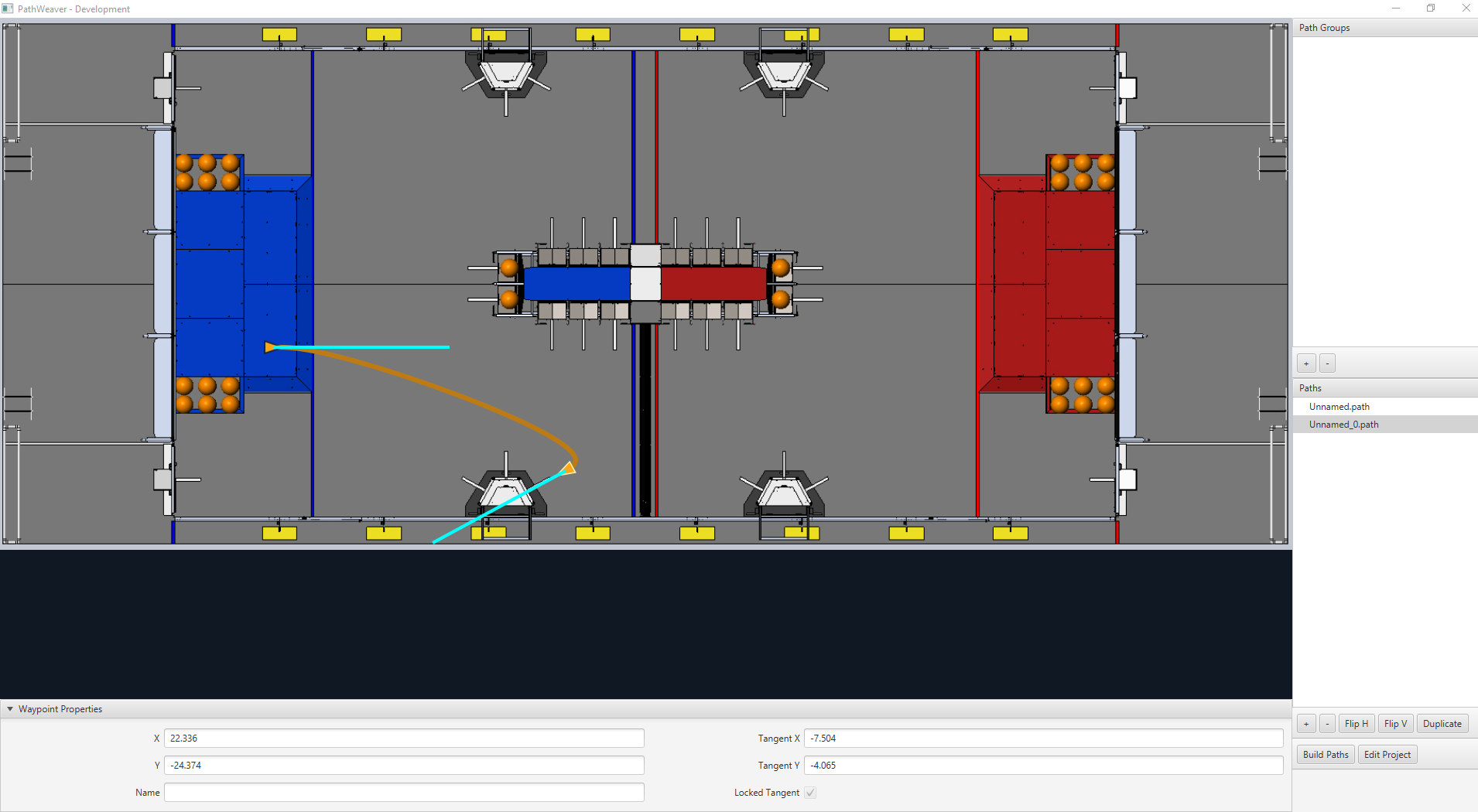
Adding Additional Waypoints to Control the Robot Path
Adding additional waypoints and changing their tangent vectors can affect the path that is followed. Additional waypoints can be added by dragging in the middle of the path. In this case, we added another waypoint in the middle of the path.

Locking the Tangent Lines
Locking tangent lines prevents them from changing when the trajectory is being manipulated. The tangent lines will also be locked when the point is moved.
More Precise control of Waypoints
While PathWeaver makes it simple to draw trajectories that the robot should follow, it is sometimes hard to precisely set where the waypoints should be placed. In this case, setting the waypoint locations can be done by entering the X and Y value which might come from an accurate CAD model of the field. The points can be entered in the X and Y fields when a waypoint is selected.
Creating Path Groups
Path Groups are a way of visualizing where one path ends and the next one starts. An example is when the robot program drives one path, does something after the path has completed, drives to another location to obtain a game piece, then back again to score it. It’s important that the start and end points of each path in the group have common end and start points. By adding all the paths to a single path group and selecting the group, all paths in that group will be shown. Then each path can be edited while viewing all the paths.
Creating a Path Group
Press the “plus” button underneath Path Groups. Then drag the Paths from the Paths section into your Path Group.
Each path added to a path group will be drawn in a different color making it easy to figure out what the name is for each path.
If there are multiple paths in a group, selection works as follows:
Selecting the group displays all paths in the group making it easy to see the relationship between them. Any waypoint on any of the paths can be edited while the group is selected and it will only change the path containing the waypoint.
Selecting on a single path in the group will only display that path, making it easy to precisely see what all the waypoints are doing and preventing clutter in the interface if multiple paths cross over or are close to each other.
Importing a PathWeaver JSON
The TrajectoryUtil class can be used to import a PathWeaver JSON into robot code to follow it. This article will go over importing the trajectory. Please visit the end-to-end trajectory tutorial for more information on following the trajectory.
The fromPathweaverJson (Java) / FromPathweaverJson (C++) static methods in TrajectoryUtil can be used to create a trajectory from a JSON file stored on the roboRIO file system.
Important
To be compatible with the Field2d view in the simulator GUI, the coordinates for the exported JSON have changed. Previously (before 2021), the range of the y-coordinate was from -27 feet to 0 feet whereas now, the range of the y-coordinate is from 0 feet to 27 feet (with 0 being at the bottom of the screen and 27 feet being at the top). This should not affect teams who are correctly resetting their odometry to the starting pose of the trajectory before path following.
Note
PathWeaver places JSON files in src/main/deploy/paths which will automatically be placed on the roboRIO file system in /home/lvuser/deploy/paths and can be accessed using getDeployDirectory as shown below.
String trajectoryJSON = "paths/YourPath.wpilib.json";
Trajectory trajectory = new Trajectory();
@Override
public void robotInit() {
try {
Path trajectoryPath = Filesystem.getDeployDirectory().toPath().resolve(trajectoryJSON);
trajectory = TrajectoryUtil.fromPathweaverJson(trajectoryPath);
} catch (IOException ex) {
DriverStation.reportError("Unable to open trajectory: " + trajectoryJSON, ex.getStackTrace());
}
}
#include <frc/Filesystem.h>
#include <frc/trajectory/TrajectoryUtil.h>
#include <wpi/fs.h>
frc::Trajectory trajectory;
void Robot::RobotInit() {
fs::path deployDirectory = frc::filesystem::GetDeployDirectory();
deployDirectory = deployDirectory / "paths" / "YourPath.wpilib.json";
trajectory = frc::TrajectoryUtil::FromPathweaverJson(deployDirectory.string());
}
In the examples above, YourPath should be replaced with the name of your path.
Warning
Loading a PathWeaver JSON from file in Java can take more than one loop iteration so it is highly recommended that the robot load these paths on startup.
Adding field images to PathWeaver
Here are instructions for adding your own field image using the 2019 game as an example.
Games are loaded from the ~/PathWeaver/Games on Linux and macOS or %USERPROFILE%/PathWeaver/Games directory on Windows. The files can be in either a game-specific subdirectory, or in a zip file in the Games directory. The ZIP file must follow the same layout as a game directory; the JSON file must be in the root of the ZIP file (cannot be in a subdirectory).
Download the example FIRST Destination Deep Space field definition here. Other field definitions are available in the PathWeaver GitHub repository.
File Layout
~/PathWeaver
/Games
/Custom Game
custom-game.json
field-image.png
OtherGame.zip
JSON Format
{
"game": "game name",
"field-image": "relative/path/to/img.png",
"field-corners": {
"top-left": [x, y],
"bottom-right": [x, y]
},
"field-size": [width, length],
"field-unit": "unit name"
}
The path to the field image is relative to the JSON file. For simplicity, the image file should be in the same directory as the JSON file.
The field corners are the X and Y coordinates of the top-left and bottom-right pixels defining the rectangular boundary of the playable area in the field image. Non-rectangular playing areas are not supported.
The field size is the width and length of the playable area of the field in the provided units.
The field units are case-insensitive and can be in meters, cm, mm, inches, feet, yards, or miles. Singular, plural, and abbreviations are supported (e.g. “meter”,”meters”, and”m”are all valid for specifying meters)
Note
When making a new field image, a border (minimum of 20 pixels is recommended) should be left around the outside so that waypoints on the field edge are accessible.
roboRIO
roboRIO Introduction
The roboRIO is designed specifically with FIRST in mind. The roboRIO has a basic architecture of a Real-Time processors + FPGA (field programmable gate array) but is more powerful, lighter, and smaller than some similar systems used in industry.
The roboRIO is a reconfigurable robotics controller that includes built-in ports for inter-integrated circuits (I2C), serial peripheral interfaces (SPI), RS232, USB, Ethernet, pulse width modulation (PWM), and relays to quickly connect the common sensors and actuators used in robotics. The controller features LEDs, buttons, an onboard accelerometer, and a custom electronics port. It has an onboard dual-core ARM real-time Cortex‑A9 processor and customizable Xilinx FPGA.
Detailed information on the roboRIO can be found in the roboRIO User Manual and in the roboRIO technical specifications.
Before deploying programs to your roboRIO, you must first image the roboRIO with the FRC roboRIO Imaging Tool.
roboRIO 2.0 microSD Card Imaging
Note
The imaging instructions for the NI roboRIO 1.0 are here.
The NI roboRIO 2.0 boots from a microSD card configured with an appropriate boot image containing the NI Linux Real-Time OS, drivers, and libraries specific to FRC. There are two ways to create the microSD card – with the roboRIO using the imaging tool, or with a laptop and an SD burner application per the instructions on this page.
Important
The first time a roboRIO 2 is imaged (or if the microSD card is replaced with a new card), it must be imaged using these instructions.
microSD Requirements
The NI roboRIO 2.0 supports all microSD cards. It is recommended to use a card with 2GB or more of capacity.
Operation Tips
The NI roboRIO 2.0 requires a fully inserted microSD card containing a valid image in order to boot and operate as intended.
If the microSD card is removed while powered, the roboRIO will hang. Once the microSD card is replaced, the roboRIO will need to be restarted using the reset button, or be power cycled.
No damage will result from microSD card removal or insertion while powered, but best practice is to perform these operations while unpowered.
Imaging Directly to the microSD Card
The image will be transferred to the microSD card using a specialized writing utility, sometimes called a burner. Several utilities are listed below, but most tools that can write arbitrary images for booting a Raspberry Pi or similar dev boards will also produce a bootable SD card for roboRIO 2.0.
Supported image files are named FRC_roboRIO2_VERSION.img.zip. You can locate them by clicking the SD button in the roboRIO Imaging tool. It is generally best to use the latest version of the image.
If using a non Windows OS you will need to copy this image file to that computer.
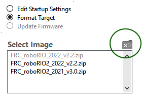
A microSD to USB dongle works well for writing to microSD cards.
Note
Raspberry Pi images will not boot on a roboRIO because the OS and drivers are incompatible. Similarly, a roboRIO image is not compatible with Raspberry Pi controller boards.
Writing the image with balenaEtcher
Download and install balenaEtcher.
Launch
Flash from file -> locate the image file you want to copy to the microSD card
Select target -> select the destination microSD device
Press Flash
Writing the image with Raspberry Pi Imager
Download and install from Raspberry Pi Imager.
Launch
Choose OS -> Use Custom -> select the image file you want to copy to the microSD card
Choose Storage -> select the destination microSD device
Press Write
Setting the roboRIO Team Number
The image writing process above does not set a team number. To fix this teams will need to insert the microSD card in the robRIO and connect to the robot. With the roboRIO Imaging Tool go to Edit Startup Settings. Next, fill out the Team Number box and hit Apply.
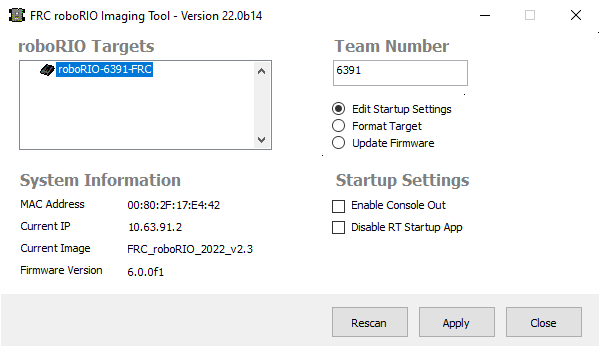
roboRIO Web Dashboard
The roboRIO web dashboard is a webpage built into the roboRIO that can be used for checking status and updating settings of the roboRIO.
Users may encounter issues using IE (compatibility) or Edge (mDNS site access). Alternate browsers such as Google Chrome or Mozilla Firefox are recommended for the best experience.
Opening the WebDash
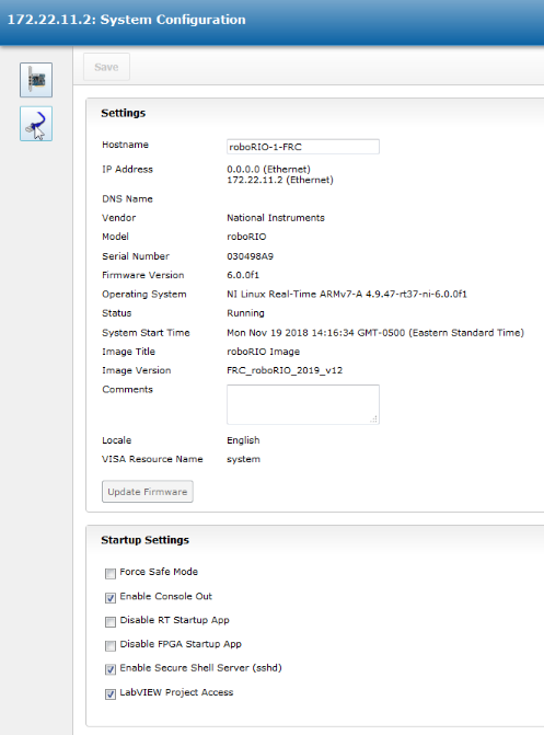
To open the web dashboard, open a web browser and enter the address of the roboRIO into the address bar (172.22.11.2 for USB, or “roboRIO-####-FRC.local where #### is your team number, with no leading zeroes, for either interface). See this document for more details about mDNS and roboRIO networking: IP Configurations
System Configuration Tab
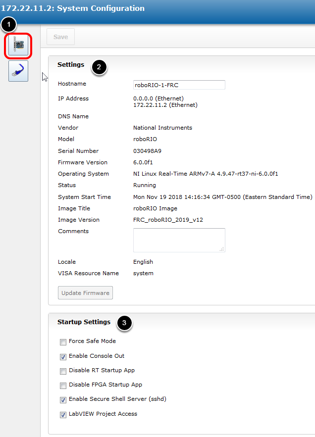
The home screen of the web dashboard is the System Configuration tab which has 5 main sections:
Navigation Bar - This section allows you to navigate to different sections of the web dashboard. The different pages accessible through this navigation bar are discussed below.
System Settings - This section contains information about the System Settings. The Hostname field should not be modified manually, instead use the roboRIO Imaging tool to set the Hostname based on your team number. This section contains information such as the device IP, firmware version and image version.
Startup Settings - This section contains Startup settings for the roboRIO. These are described in the sub-step below
System Resources (not pictured) - This section provides a snapshot of system resources such as memory and CPU load.
Startup Settings
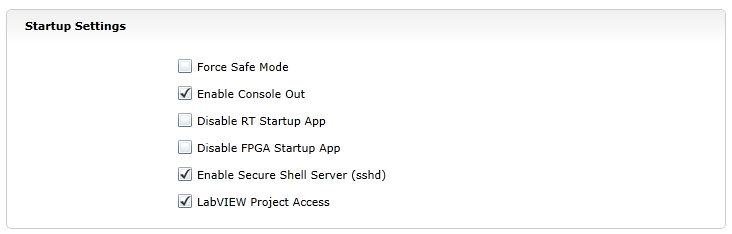
Force Safe Mode - Forces the controller into Safe Mode. This can be used with troubleshooting imaging issues, but it is recommended to use the Reset button on the roboRIO to put the device into Safe Mode instead (with power already applied, hold the rest button for 5 seconds). Default is unchecked.
Enable Console Out - This enables the on-board RS232 port to be used as a Console output. It is recommended to leave this enabled unless you are using this port to talk to a serial device (note that this port uses RS232 levels and and should not be connected to many microcontrollers which use TTL levels). Default is checked.
Disable RT Startup App - Checking this box disables code from running at startup. This may be used for troubleshooting if you find the roboRIO is unresponsive to new program download. Default is unchecked
Disable FPGA Startup App - This box should not be checked.
Enable Secure Shell Server (sshd) - It is recommended to leave this box checked. This setting enables SSH which is a way to remotely access a console on the roboRIO. Unchecking this box will prevent C++ and Java teams from loading code onto the roboRIO.
LabVIEW Project Access -** It is recommended to leave this box checked.** This setting allows LabVIEW projects to access the roboRIO.
Network Configuration
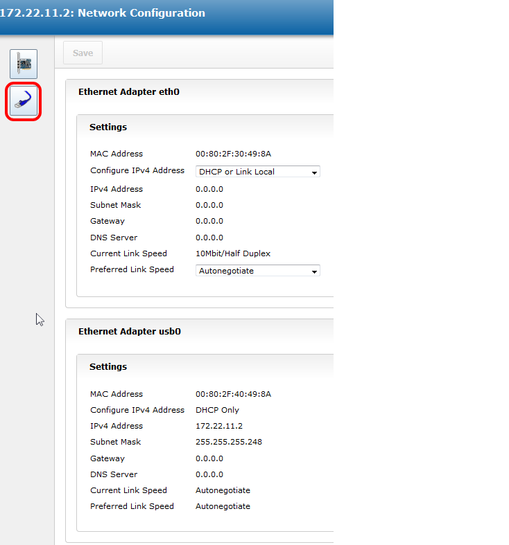
This page shows the configuration of the roboRIO’s network adapters. It is not recommended to change any settings on this page. For more information on roboRIO networking see this article: IP Configurations
roboRIO FTP
Note
The roboRIO has both SFTP and anonymous FTP enabled. This article describes how to use each to access the roboRIO file system.
SFTP
SFTP is the recommended way to access the roboRIO file system. Because you will be using the same account that your program will run under, files copied over should always have permissions compatible with your code.
Software
There are a number of freely available programs for SFTP. This article will discuss using FileZilla. You can either download and install FileZilla before proceeding or extrapolate the directions below to your SFTP client of choice.
Connecting to the roboRIO
To connect to your roboRIO:
Enter the mDNS name (roboRIO-TEAM-frc.local) in the “Host” box
Enter “lvuser” in the Username box (this is the account your program runs under)
Leave the Password box blank
Enter “22” in the port box (the SFTP default port)
Click Quickconnect
Browsing the roboRIO filesystem
After connecting to the roboRIO, Filezilla will open to the \home\lvuser directory. The right pane is the remote system (the roboRIO), the left pane is the local system (your computer). The top section of each pane shows you the hierarchy to the current directory you are browsing, the bottom pane shows contents of the directory. To transfer files, simply click and drag from one side to the other. To create directories on the roboRIO, right click and select “Create Directory”.
FTP
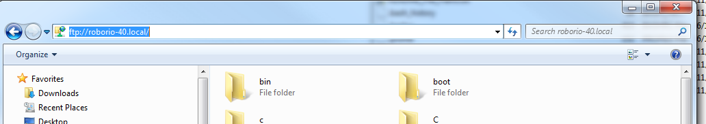
The roboRIO also has anonymous FTP enabled. It is recommended to use SFTP as described above, but depending on what you need FTP may work in a pinch with no additional software required. To FTP to the roboRIO, open a Windows Explorer window (on Windows 7, you can click Start->My Computer). In the address bar, type ftp://roboRIO-TEAM-frc.local and press enter. You can now browse the roboRIO file system just like you would browse files on your computer.
roboRIO User Accounts and SSH
Note
This document contains advanced topics not required for typical FRC® programming
The roboRIO image contains a number of accounts, this article will highlight the two used for FRC and provide some detail about their purpose. It will also describe how to connect to the roboRIO over SSH.
roboRIO User Accounts
The roboRIO image contains a number of user accounts, but there are two of primary interest for FRC.
Admin
The “admin” account has root access to the system and can be used to manipulate OS files or settings. Teams should take caution when using this account as it allows for the modification of settings and files that may corrupt the operating system of the roboRIO. The credentials for this account are:
Username: admin
Password:
Note
The password is intentionally blank.
Lvuser
The “lvuser” account is the account used to run user code for all three languages. The credentials for this account should not be changed. Teams may wish to use this account (via ssh or sftp) when working with the roboRIO to ensure that any files or settings changes are being made on the same account as their code will run under.
Danger
Changing the default ssh passwords for either “lvuser” or “admin” will prevent C++ and Java teams from uploading code.
SSH
SSH (Secure SHell) is a protocol used for secure data communication. When broadly referred to regarding a Linux system (such as the one running on the roboRIO) it generally refers to accessing the command line console using the SSH protocol. This can be used to execute commands on the remote system. A free client which can be used for SSH is PuTTY: https://www.chiark.greenend.org.uk/~sgtatham/putty/latest.html
Open Putty
Open Putty (clicking OK at any security prompt). Then set the following settings:
Host Name: roboRIO-TEAM-frc.local (where TEAM is your team number, example shows team 40)
Connection Type: SSH
Other settings can be left at defaults. Click Open to open the connection. If you see a prompt about SSH keys, click OK.
If you are connected over USB you can use 172.22.11.2 as the hostname. If your roboRIO is set to a static IP you can use that IP as the hostname if connected over Ethernet/wireless.
Log In
When you see the prompt, enter the desired username (see above for description) then press enter. At the password prompt press enter (password for both accounts is blank).
roboRIO Brownout and Understanding Current Draw
In order to help maintain battery voltage to preserve itself and other control system components such as the radio during high current draw events, the roboRIO contains a staged brownout protection scheme. This article describes this scheme, provides information about proactively planning for system current draw, and describes how to use the new functionality of the PDP as well as the DS Log File Viewer to understand brownout events if they do happen on your robot.
roboRIO Brownout Protection
The roboRIO uses a staged brownout protection scheme to attempt to preserve the input voltage to itself and other control system components in order to prevent device resets in the event of large current draws pulling the battery voltage dangerously low.
Stage 1 - 6v output drop
Voltage Trigger - 6.8V
When the voltage drops below 6.8V, the 6V output on the PWM pins will start to drop.
Stage 2 - Output Disable
Voltage Trigger - 6.3V
When the voltage drops below 6.3V, the controller will enter the brownout protection state. The following indicators will show that this condition has occurred:
Power LED on the roboRIO will turn Amber
Background of the voltage display on the Driver Station will turn red
Mode display on the Driver Station will change to Voltage Brownout
The CAN/Power tab of the DS will increment the 12V fault counter by 1.
The DS will record a brownout event in the DS log.
The controller will take the following steps to attempt to preserve the battery voltage:
PWM outputs will be disabled. For PWM outputs which have set their neutral value (all motor controllers in WPILib) a single neutral pulse will be sent before the output is disabled.
6V, 5V, 3.3V User Rails disabled (This includes the 6V outputs on the PWM pins, the 5V pins in the DIO connector bank, the 5V pins in the Analog bank, the 3.3V pins in the SPI and I2C bank and the 5V and 3.3V pins in the MXP bank)
GPIO configured as outputs go to High-Z
Relay Outputs are disabled (driven low)
CAN-based motor controllers are sent an explicit disable command
Pneumatic Devices such as the CTRE Pneumatics Control Module and REV Pneumatic Hub are disabled
The controller will remain in this state until the voltage rises to greater than 7.5V or drops below the trigger for the next stage of the brownout
Stage 3 - Device Blackout
Voltage Trigger - 4.5V
Below 4.5V the device may blackout. The exact voltage may be lower than this and depends on the load on the device.
The controller will remain in this state until the voltage rises above 4.65V when the device will begin the normal boot sequence.
Avoiding Brownout - Proactive Current Draw Planning
The key to avoiding a brownout condition is to proactively plan for the current draw of your robot. The best way to do this is to create some form of power budget. This can be a complex document that attempts to quantify both estimated current draw and time in an effort to most completely understand power usage and therefore battery state at the end of a match, or it can be a simple inventory of current usage. To do this:
Establish the max “sustained” current draw (with sustained being loosely defined here as not momentary). This is probably the most difficult part of creating the power budget. The exact current draw a battery can sustain while maintaining a voltage of 7+ volts is dependent on a variety of factors such as battery health (see this article for measuring battery health) and state of charge. As shown in the NP18-12 data sheet, the terminal voltage chart gets very steep as state of charge decreases, especially as current draw increases. This datasheet shows that at 3CA continuous load (54A) a brand new battery can be continuously run for over 6 minutes while maintaining a terminal voltage of over 7V. As shown in the image above (used with permission from Team 234s Drive System Testing document), even with a fresh battery, drawing 240A for more than a second or two is likely to cause an issue. This gives us some bounds on setting our sustained current draw. For the purposes of this exercise, we’ll set our limit at 180A.
List out the different functions of your robot such as drivetrain, manipulator, main game mechanism, etc.
Start assigning your available current to these functions. You will likely find that you run out pretty quickly. Many teams gear their drivetrain to have enough torque to slip their wheels at 40-50A of current draw per motor. If we have 4 motors on the drivetrain, that eats up most, or even exceeds, our power budget! This means that we may need to put together a few scenarios and understand what functions can (and need to be) be used at the same time. In many cases, this will mean that you really need to limit the current draw of the other functions if/while your robot is maxing out the drivetrain (such as trying to push something). Benchmarking the “driving” current requirements of a drivetrain for some of these alternative scenarios is a little more complex, as it depends on many factors such as number of motors, robot weight, gearing, and efficiency. Current numbers for other functions can be done by calculating the power required to complete the function and estimating efficiency (if the mechanism has not been designed) or by determining the torque load on the motor and using the torque-current curve to determine the current draw of the motors.
If you have determined mutually exclusive functions in your analysis, consider enforcing the exclusion in software. You may also use the current monitoring of the PDP (covered in more detail below) in your robot program to provide output limits or exclusions dynamically (such as don’t run a mechanism motor when the drivetrain current is over X or only let the motor run up to half output when the drivetrain current is over Y).
Settable Brownout
The NI roboRIO 1.0 does not support custom brownout voltages. It is fixed at 6.3V as mentioned in Stage 2 above.
The NI roboRIO 2.0 adds the option for a software settable brownout level. The default brownout level (Stage 2) of the roboRIO 2.0 is 6.75V.
RobotController.setBrownoutVoltage(7.0);
frc::RobotController::SetBrownoutVoltage(7_V);
Measuring Current Draw using the PDP/PDH
The FRC® Driver Station works in conjunction with the roboRIO and PDP/PDH to extract logged data from the PDP/PDH and log it on your DS PC. A viewer for this data is still under development.
In the meantime, teams can use their robot code and manual logging, a LabVIEW front panel or the SmartDashboard to visualize current draw on their robot as mechanisms are developed. In LabVIEW, you can read the current on a PDP/PDH channel using the Get PD Currents VI found on the Power pallet. For C++ and Java teams, use the PowerDistribution class as described in the Power Distribution article. Plotting this information over time (easiest with a LV Front Panel or with the SmartDashboard by using a Graph indicator can provide information to compare against and update your power budget or can locate mechanisms which do not seem to be performing as expected (due to incorrect load calculation, incorrect efficiency assumptions, or mechanism issues such as binding).
Identifying Brownouts
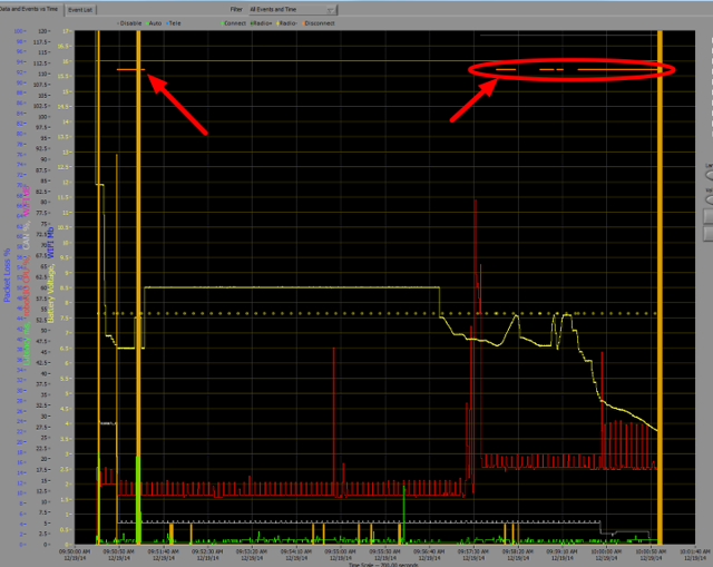
The easiest way to identify a brownout is by clicking on the CAN\Power tab of the DS and checking the 12V fault count. Alternately, you can review the Driver Station Log after the fact using the Driver Station Log Viewer. The log will identify brownouts with a bright orange line, such as in the image above (note that these brownouts were induced with a benchtop supply and may not reflect the duration and behavior of brownouts on a typical FRC robot).
Recovering a roboRIO using Safe Mode
Occasionally a roboRIO may become corrupted to the point that it cannot be recovered using the normal boot and imaging process. Booting the roboRIO into Safe Mode may allow the device to be successfully re-imaged.
Booting into Safe Mode

To boot the roboRIO into Safe Mode:
Apply power to the roboRIO
Press and hold the Reset button until the Status LED lights up (~5 seconds) then release the Reset button
The roboRIO will boot in Safe Mode (indicated by the Status LED flashing in groups of 3)
Recovering the roboRIO
The roboRIO can now be imaged by using the roboRIO Imaging Tool as described in Imaging your roboRIO.
About Safe Mode
In Safe Mode, the roboRIO boots a separate copy of the operating system into a RAM Disk. This allows you to recover the roboRIO even if the normal copy of the OS is corrupted. While in Safe Mode, any changes made to the OS (such as changes made by accessing the device via SSH or Serial) will not persist to the normal copy of the OS stored on disk.
Advanced GradleRIO
GradleRIO is the mechanism that powers the deployment of robot code to the roboRIO. GradleRIO is built on the popular Gradle dependency and build management system. This section highlights advanced configurations that teams can use to enhance their workflow.
Using External Libraries with Robot Code
Warning
Using external libraries may have unintended behavior with your robot code! It is not recommended unless you are aware of what you are doing!
Often a team might want to add external Java or C++ libraries for usage with their robot code. This article highlights adding Java libraries to your Gradle dependencies, or the options that C++ teams have.
Java
Note
Any external dependencies that rely on native libraries (JNI) are likely not going to work.
Java is quite simple to add external dependencies. You simply add the required repositories and dependencies.
Robot projects by default do not have a repositories {} block in the build.gradle file. You will have to add this yourself. Above the dependencies {} block, please add the following:
repositories {
mavenCentral()
...
}
mavenCentral() can be replaced with whatever repository the library you want to import is using. Now you have to add the dependency on the library itself. This is done by adding the necessary line to your dependencies {} block. The below example showcases adding Apache Commons to your Gradle project.
dependencies {
implementation 'org.apache.commons:commons-lang3:3.6'
...
}
Now you run a build and ensure the dependencies are downloaded. Intellisense may not work properly until a build is ran!
C++
Adding C++ dependencies to your robot project is non-trivial due to needing to compile for the roboRIO. You have a couple of options.
Copy the source code of the wanted library into your robot project.
Use the vendordep template as an example and create a vendordep.
Copying Source Code
Simply copy the necessary source and/or headers into your robot project. You can then configure any necessary platform args like below:
nativeUtils.platformConfigs.named("linuxx86-64").configure {
it.linker.args.add('-lstdc++fs') // links in C++ filesystem library
}
Creating a Vendordep
Please follow the instructions in the vendordep repository.
Setting up CI for Robot Code using GitHub Actions
An important aspect of working in a team environment is being able to test code that is pushed to a central repository such as GitHub. For example, a project manager or lead developer might want to run a set of unit tests before merging a pull request or might want to ensure that all code on the main branch of a repository is in working order.
GitHub Actions is a service that allows for teams and individuals to build and run unit tests on code on various branches and on pull requests. These types of services are more commonly known as “Continuous Integration” services. This tutorial will show you how to setup GitHub Actions on robot code projects.
Note
This tutorial assumes that your team’s robot code is being hosted on GitHub. For an introduction to Git and GitHub, please see this introduction guide.
Creating the Action
The instructions for carrying out the CI process are stored in a YAML file. To create this, click on the “Actions” tab at the top of your repository. Then click on the “set up a workflow yourself” hyperlink.
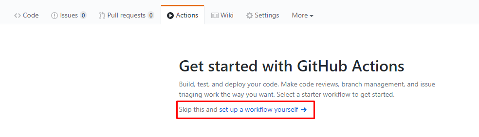
You will now be greeted with a text editor. Replace all the default text with the following:
# This is a basic workflow to build robot code.
name: CI
# Controls when the action will run. Triggers the workflow on push or pull request
# events but only for the main branch.
on:
push:
branches: [ main ]
pull_request:
branches: [ main ]
# A workflow run is made up of one or more jobs that can run sequentially or in parallel
jobs:
# This workflow contains a single job called "build"
build:
# The type of runner that the job will run on
runs-on: ubuntu-latest
# This grabs the WPILib docker container
container: wpilib/roborio-cross-ubuntu:2022-18.04
# Steps represent a sequence of tasks that will be executed as part of the job
steps:
# Checks-out your repository under $GITHUB_WORKSPACE, so your job can access it
- uses: actions/checkout@v2
# Grant execute permission for gradlew
- name: Grant execute permission for gradlew
run: chmod +x gradlew
# Runs a single command using the runners shell
- name: Compile and run tests on robot code
run: ./gradlew build
Then, save changes by clicking the “Start commit” button on the top-right corner of the screen. You can amend the default commit message if you wish to do so. Then, click the green “Commit new file” button.
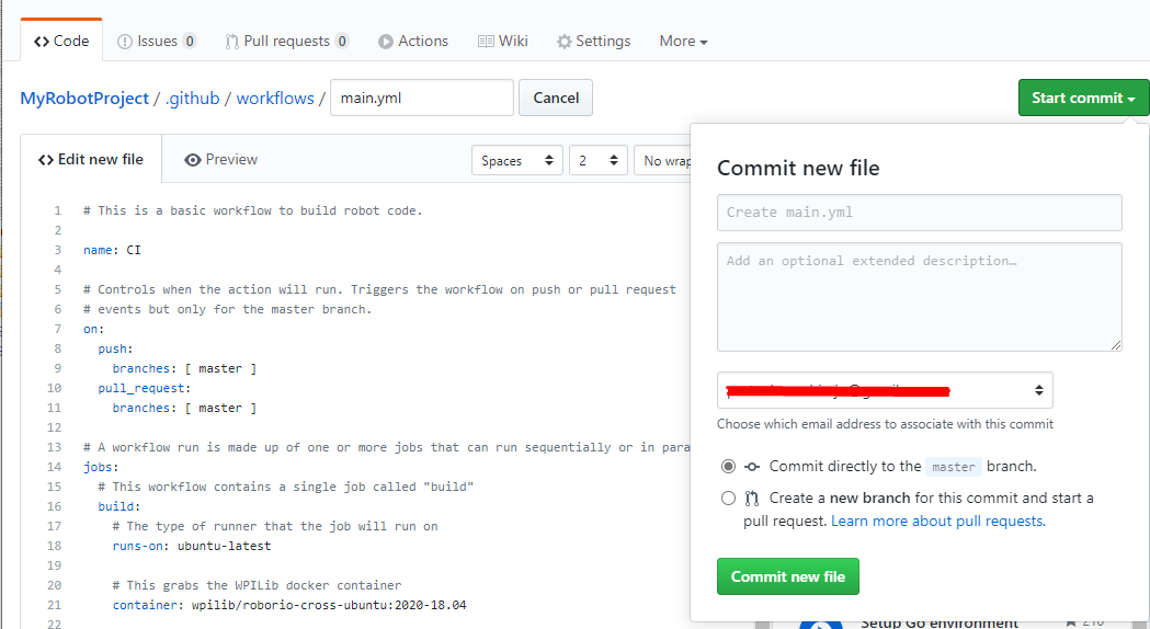
GitHub will now automatically run a build whenever a commit is pushed to main or a pull request is opened. To monitor the status of any build, you can click on the “Actions” tab on the top of the screen.
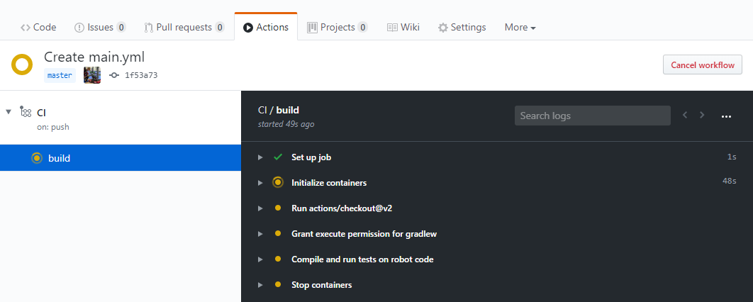
A Breakdown of the Actions YAML File
Here is a breakdown of the YAML file above. Although a strict understanding of each line is not required, some level of understanding will help you add more features and debug potential issues that may arise.
# Controls when the action will run. Triggers the workflow on push or pull request
# events but only for the main branch.
on:
push:
branches: [ main ]
pull_request:
branches: [ main ]
This block of code dictates when the Action will run. Currently, the action will run when commits are pushed to main or when pull requests are opened against main.
# A workflow run is made up of one or more jobs that can run sequentially or in parallel
jobs:
# This workflow contains a single job called "build"
build:
# The type of runner that the job will run on
runs-on: ubuntu-latest
# This grabs the WPILib docker container
container: wpilib/roborio-cross-ubuntu:2022-18.04
Each Action workflow is made of a one or more jobs that run either sequentially (one after another) or in parallel (at the same time). In our workflow, there is only one “build” job.
We specify that we want the job to run on an Ubuntu virtual machine and in a virtualized Docker container that contains the JDK, C++ compiler and roboRIO toolchains.
# Steps represent a sequence of tasks that will be executed as part of the job
steps:
# Checks-out your repository under $GITHUB_WORKSPACE, so your job can access it
- uses: actions/checkout@v2
# Grant execute permission for gradlew
- name: Grant execute permission for gradlew
run: chmod +x gradlew
# Runs a single command using the runners shell
- name: Compile and run tests on robot code
run: ./gradlew build
Each job has certain steps that will be executed. This job has three steps. The first step involves checking out the repository to access the robot code. The second step involves giving the virtual machine permission to execute gradle tasks using ./gradlew. The final step runs ./gradlew build to compile robot code and run any unit tests.
Adding a Build Status Badge to a README.md File
It is helpful to add a CI status badge to the top of your repository’s README file to quickly check the status of the latest build on main. To do this, click on the “Actions” tab at the top of the screen and select the “CI” tab on the left side of the screen. Then, click on the “Create status badge” button on the top right and copy the status badge Markdown code.
Finally, paste the Markdown code you copied at the top of your README file, commit, and push your changes. Now, you should see the GitHub Actions status badge on your main repository page.
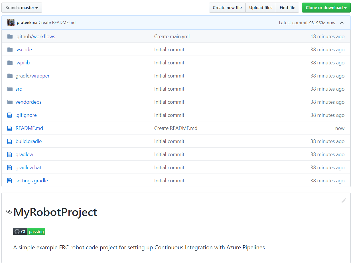
Using a Code Formatter
Code formatters exist to ensure that the style of code written is consistent throughout the entire codebase. This is used in many major projects; from Android to OpenCV. Teams may wish to add a formatter throughout their robot code to ensure that the codebase maintains readability and consistency throughout.
For this article, we will highlight using Spotless for Java teams and wpiformat for C++ teams.
Spotless
Configuration
Necessary build.gradle changes are required to get Spotless functional. In the plugins {} block of your build.gradle, add the Spotless plugin so it appears similar to the below.
plugins {
id "java"
id "edu.wpi.first.GradleRIO" version "2022.1.1"
id 'com.diffplug.spotless' version '6.1.0'
}
Then ensure you add a required spotless {} block to correctly configure spotless. This can just get placed at the end of your build.gradle.
spotless {
java {
target fileTree('.') {
include '**/*.java'
exclude '**/build/**', '**/build-*/**'
}
toggleOffOn()
googleJavaFormat()
removeUnusedImports()
trimTrailingWhitespace()
endWithNewline()
}
groovyGradle {
target fileTree('.') {
include '**/*.gradle'
exclude '**/build/**', '**/build-*/**'
}
greclipse()
indentWithSpaces(4)
trimTrailingWhitespace()
endWithNewline()
}
format 'xml', {
target fileTree('.') {
include '**/*.xml'
exclude '**/build/**', '**/build-*/**'
}
eclipseWtp('xml')
trimTrailingWhitespace()
indentWithSpaces(2)
endWithNewline()
}
format 'misc', {
target fileTree('.') {
include '**/*.md', '**/.gitignore'
exclude '**/build/**', '**/build-*/**'
}
trimTrailingWhitespace()
indentWithSpaces(2)
endWithNewline()
}
}
Running Spotless
Spotless can be ran using ./gradlew spotlessApply which will apply all formatting options. You can also specify a specific task by just adding the name of formatter. An example is ./gradlew spotlessmiscApply.
Spotless can also be used as a CI check. The check is ran with ./gradlew spotlessCheck.
Explanation of Options
Each format section highlights formatting of custom files in the project. The java and groovyGradle are natively supported by spotless, so they are defined differently.
Breaking this down, we can split this into multiple parts.
Formatting Java
Formatting Gradle files
Formatting XML files
Formatting Miscellaneous files
They are all similar, except for some small differences that will be explained. The below example will highlight the java {} block.
java {
target fileTree('.') {
include '**/*.java'
exclude '**/build/**', '**/build-*/**'
}
toggleOffOn()
googleJavaFormat()
removeUnusedImports()
trimTrailingWhitespace()
endWithNewline()
}
Let’s explain what each of the options mean.
target fileTree('.') {
include '**/*.java'
exclude '**/build/**', '**/build-*/**'
}
The above example tells spotless where our Java classes are and to exclude the build directory. The rest of the options are fairly self-explanatory.
toggleOffOn()adds the ability to have spotless ignore specific portions of a project. The usage looks like the following
// format:off
public void myWeirdFunction() {
}
// format:on
googleJavaFormat()tells spotless to format according to the Google Style GuideremoveUnusedImports()will remove any unused imports from any of your java classestrimTrailingWhitespace()will remove any extra whitespace at the end of your linesendWithNewline()will add a newline character to the end of your classes
In the groovyGradle block, there is a greclipse option. This is the formatter that spotless uses to format gradle files.
Additionally, there is a eclipseWtp option in the xml block. This stands for “Gradle Web Tools Platform” and is the formatter to format xml files. Teams not using any XML files may wish to not include this configuration.
Note
A full list of configurations is available on the Spotless README
Issues with Line Endings
Spotless will attempt to apply line endings per-OS, which means Git diffs will be constantly changing if two users are on different OSes (Unix vs Windows). It’s recommended that teams who contribute to the same repository from multiple OSes utilize a .gitattributes file. The following should suffice for handling line endings.
*.gradle text eol=lf
*.java text eol=lf
*.md text eol=lf
*.xml text eol=lf
wpiformat
Requirements
clang-format (included with LLVM)
Important
Windows is not currently supported at this time! Installing LLVM with Clang will break normal robot builds if installed on Windows.
You can install wpiformat by typing pip3 install wpiformat into a terminal or command prompt.
Usage
wpiformat can be ran by typing wpiformat in a console. This will format with clang-format. Three configuration files are required (.clang-format, .styleguide, .styleguide-license). These must exist in the project root.
An example styleguide is shown below:
cppHeaderFileInclude {
\.h$
\.hpp$
\.inc$
\.inl$
}
cppSrcFileInclude {
\.cpp$
}
modifiableFileExclude {
gradle/
}
Note
Teams can adapt .styleguide and .styleguide-license however they wish. It’s important that these are not deleted, as they are required to run wpiformat!
You can turn this into a CI check by running git --no-pager diff --exit-code HEAD. It can be configured with a .clang-format configuration file. An example configuration file is provided below.
Below is an example GitHub Actions check that uses wpiformat
wpiformat:
name: "wpiformat"
runs-on: ubuntu-latest
steps:
- uses: actions/checkout@v2
- name: Fetch all history and metadata
run: |
git fetch --prune --unshallow
git checkout -b pr
git branch -f main origin/main
- name: Set up Python 3.8
uses: actions/setup-python@v2
with:
python-version: 3.8
- name: Install clang-format
run: sudo apt-get update -q && sudo apt-get install -y clang-format-12
- name: Install wpiformat
run: pip3 install wpiformat
- name: Run
run: wpiformat -clang 12
- name: Check Output
run: git --no-pager diff --exit-code HEAD
Gradlew Tasks
This article aims to highlight the gradle commands supported by the WPILib team for user use. These commands can be viewed by typing ./gradlew tasks at the root of your robot project. Not all commands shown in ./gradlew tasks and unsupported commands will not be documented here.
Build tasks
./gradlew build - Assembles and tests this project. Useful for prebuilding your project without deploying to the roboRIO.
./gradlew clean - Deletes the build directory.
CompileCommands tasks
./gradlew generateCompileCommands - Generate compile_commands.json. This is a configuration file that is supported by many Integrated Development Environments.
EmbeddedTools tasks
./gradlew deploy - Deploy all artifacts on all targets. This will deploy your robot project to the available targets (IE, roboRIO).
./gradlew discoverRoborio - Determine the address(es) of target RoboRIO. This will print out the IP address of a connected roboRIO.
GradleRIO tasks
./gradlew downloadAll - Download all dependencies that may be used by this project
./gradlew $TOOL$ - Runs the tool $TOOL$ (Replace $TOOL$ with the name of the tool. IE, Glass, Shuffleboard, etc)
./gradlew $TOOL$Install - Installs the tool $TOOL$ (Replace $TOOL$ with the name of the tool. IE, Glass, Shuffleboard, etc)
./gradlew InstallAllTools - Installs all available tools. This excludes the development environment such as VSCode. It’s the users requirement to ensure the required dependencies (Java) is installed. Only recommended for advanced users!
./gradlew riolog - Runs a console displaying output from the default RoboRIO (roborio)
./gradlew simulateExternalCpp - Simulate External Task for native executable. Exports a JSON file for use by editors / tools
./gradlew simulateExternalJava - Simulate External Task for Java/Kotlin/JVM. Exports a JSON file for use by editors / tools
./gradlew simulateJava - Launches simulation for the Java projects
./gradlew simulateNative - Launches simulation for C++ projects
./gradlew vendordep - Install vendordep JSON file from URL or local installation. See 3rd Party Libraries
Including Git Data in Deploy
This article will go over how to include information from Git, such as branch name or commit hash, into the robot code. This is necessary for using such information in robot code, such as printing out commit hash and branch name when the robot starts.
Note
Git must be in the path for this to work. This should be enabled by default when installing Git.
Deploying Branch Name
This example uses git rev-parse to extract data the name of the current branch. The Git command used for this is:
$ git rev-parse --abbrev-ref HEAD
The --abbrev-ref flag tells Git to use a short version of the name for the current commit that rev-parse is acting on. When HEAD is the most recent commit on a branch, this will return the name of that branch.
Next, create a new task in the build.gradle file that will run the above Git command and write it to a file in the src/main/deploy directory. For example, the following is an example task named writeBranchName that will write the branch name to a file named branch.txt.
tasks.register("writeBranchName") {
// Define an output stream to write to instead of terminal
def stdout = new ByteArrayOutputStream()
// Execute the git command
exec {
commandLine "git", "rev-parse", "--abbrev-ref", "HEAD"
// Write to the output stream instead of terminal
standardOutput = stdout
}
// Parse the output into a string
def branch = stdout.toString().trim()
// Create a new file
new File(
// Join project directory and deploy directory
projectDir.toString() + "/src/main/deploy",
// File name to write to
"branch.txt"
).text = branch // Set the contents of the file to the variable branch
}
This registers a Gradle task that uses the above Git command, saves the output to a variable, and then writes it to a file. Since it was written to the src/main/deploy directory, it will be included in the jar file deployed to the robot and accessible in code.
The next step is to make the deploy task depend on the task you created, so that it will automatically run before the code is deployed. This example uses the task name writeBranchName from the previous example, but it should be replaced with the name of the task in your build.gradle.
deploy.targets.roborio.artifacts.frcStaticFileDeploy.dependsOn(writeBranchName)
Deploying Commit Hash
Similar to the previous example, git rev-parse will be used to parse the current commit hash. The Git command used for this is:
$ git rev-parse --short HEAD
Similar to the previous Git command, rev-parse is used to find information about the commit at HEAD. However, instead of using --abbrev-ref to find the branch name associated with that commit, --short is used to find the 7-character commit hash.
Note
If you wish to use the full commit hash instead of the 7-character version, you can leave out the --short flag.
Next is to create a task in build.gradle that runs this command and writes the output to a file. This is largely the same as the first example, except the task is named writeCommitHash, the new Git command is used, and it is written to commit.txt instead of branch.txt.
tasks.register("writeCommitHash") {
def stdout = new ByteArrayOutputStream()
exec {
commandLine "git", "rev-parse", "--short", "HEAD"
standardOutput = stdout
}
def commitHash = stdout.toString().trim()
new File(
projectDir.toString() + "/src/main/deploy",
"commit.txt"
).text = commitHash
}
deploy.targets.roborio.artifacts.frcStaticFileDeploy.dependsOn(writeCommitHash)
Ignoring Generated Files with Git
Since these files include data that is already tracked by Git and are regenerated every time code is deployed, it is recommended to not track these changes with Git by using the gitignore file. This file should exist by default in any project generated by the WPILib VS Code extension. Below is an example that continues to use the branch.txt and commit.txt file names:
src/main/deploy/branch.txt
src/main/deploy/commit.txt
...
Using Deployed Files
In order to access files that were written to the deploy directory in code, you have to use the getDeployDirectory() method of the Filesystem class in Java, or the GetDeployDirectory() function of the frc::filesystem namespace in C++. Below is an example of opening both files from the previous examples:
Note
Opening and reading the files is slow and should not be performed during any periodic methods. Since the file will only change on deploy, it only needs to be read once.
File deployDir = Filesystem.getDeployDirectory();
File branchFile = new File(deployDir, "branch.txt");
File commitFile = new File(deployDir, "commit.txt");
For more information on how to interact with the file objects, see the documentation of the File class.
Advanced Controls
This section covers advanced control features in WPILib, such as various feedback/feedforward control algorithms and trajectory following.
A Video Walkthrough of Model Based Validation of Autonomous in FRC
At the “RSN Spring Conference, Presented by WPI” in 2020, Tyler Veness from the WPILib team gave a presentation on Model Based Validation of Autonomous in FRC®.
The link to the presentation is available here.
Advanced Controls Introduction
Control System Basics
Note
This article is taken out of Controls Engineering in FRC by Tyler Veness with permission.
Control systems are all around us and we interact with them daily. A small list of ones you may have seen includes heaters and air conditioners with thermostats, cruise control and the anti-lock braking system (ABS) on automobiles, and fan speed modulation on modern laptops. Control systems monitor or control the behavior of systems like these and may consist of humans controlling them directly (manual control), or of only machines (automatic control).
How can we prove closed-loop controllers on an autonomous car, for example, will behave safely and meet the desired performance specifications in the presence of uncertainty? Control theory is an application of algebra and geometry used to analyze and predict the behavior of systems, make them respond how we want them to, and make them robust to disturbances and uncertainty.
Controls engineering is, put simply, the engineering process applied to control theory. As such, it’s more than just applied math. While control theory has some beautiful math behind it, controls engineering is an engineering discipline like any other that is filled with trade-offs. The solutions control theory gives should always be sanity checked and informed by our performance specifications. We don’t need to be perfect; we just need to be good enough to meet our specifications.
Nomenclature
Most resources for advanced engineering topics assume a level of knowledge well above that which is necessary. Part of the problem is the use of jargon. While it efficiently communicates ideas to those within the field, new people who aren’t familiar with it are lost.
The system or collection of actuators being controlled by a control system is called the plant. A controller is used to drive the plant from its current state to some desired state (the reference). Controllers which don’t include information measured from the plant’s output are called open-loop controllers.
Controllers which incorporate information fed back from the plant’s output are called closed-loop controllers or feedback controllers.
Note
The input and output of a system are defined from the plant’s point of view. The negative feedback controller shown is driving the difference between the reference and output, also known as the error, to zero.
What is Gain?
Gain is a proportional value that shows the relationship between the magnitude of an input signal to the magnitude of an output signal at steady-state. Many systems contain a method by which the gain can be altered, providing more or less “power” to the system.
The figure below shows a system with a hypothetical input and output. Since the output is twice the amplitude of the input, the system has a gain of two.
Block Diagrams
When designing or analyzing a control system, it is useful to model it graphically. Block diagrams are used for this purpose. They can be manipulated and simplified systematically.
The open-loop gain is the total gain from the sum node at the input (the circle) to the output branch. this would be the system’s gain if the feedback loop was disconnected. The feedback gain is the total gain from the output back to the input sum node. A sum node’s output is the sum of its inputs.
The below figure is a block diagram with more formal notation in a feedback configuration.
\(\mp\) means “minus or plus” where a minus represents negative feedback.
Why Feedback Control?
Let’s say we are controlling a DC brushed motor. With just a mathematical model and knowledge of all the current states of the system (i.e., angular velocity), we can predict all future states given the future voltage inputs. Why then do we need feedback control? If the system is disturbed in any way that isn’t modeled by our equations, like a load was applied, or voltage sag in the rest of the circuit caused the commanded voltage to not match the applied voltage, the angular velocity of the motor will deviate from the model over time.
To combat this, we can take measurements of the system and the environment to detect this deviation and account for it. For example, we could measure the current position and estimate an angular velocity from it. We can then give the motor corrective commands as well as steer our model back to reality. This feedback allows us to account for uncertainty and be robust to it.
PID Introduction Video by WPI
Have you ever had trouble designing a robot system to move quickly and then stop at exactly a desired position? Challenges like this can arise when driving fixed distances or speeds, operating an arm or elevator, or any other motor controlled system that requires specific motion. In this video, WPI Professor Dmitry Berenson talks about robot controls and how PID controls work.
Introduction to PID
The PID controller is a commonly used feedback controller consisting of proportional, integral, and derivative terms, hence the name. This article will build up the definition of a PID controller term by term while trying to provide some intuition for how each of them behaves.
First, we’ll get some nomenclature for PID controllers out of the way. The reference is called the setpoint (the desired position) and the output is called the process variable (the measured position). Below are some common variable naming conventions for relevant quantities.
\(r(t)\) |
\(u(t)\) |
||
\(e(t)\) |
\(y(t)\) |
The error \(e(t)\) is \(r(t) - y(t)\).
For those already familiar with PID control, this book’s interpretation won’t be consistent with the classical intuition of “past”, “present”, and “future” error. We will be approaching it from the viewpoint of modern control theory with proportional controllers applied to different physical quantities we care about. This will provide a more complete explanation of the derivative term’s behavior for constant and moving setpoints.
The proportional term drives the position error to zero, the derivative term drives the velocity error to zero, and the integral term accumulates the area between the setpoint and output plots over time (the integral of position error) and adds the current total to the control input. We’ll go into more detail on each of these.
Proportional Term
The Proportional term drives the position error to zero.
where \(K_p\) is the proportional gain and \(e(t)\) is the error at the current time \(t\).
The below figure shows a block diagram for a system controlled by a P controller.
Proportional gains act like a “software-defined springs” that pull the system toward the desired position. Recall from physics that we model springs as \(F = - kx\) where \(F\) is the force applied, \(k\) is a proportional constant, and \(x\) is the displacement from the equilibrium point. This can be written another way as \(F = k(0-x)\) where \(0\) is the equilibrium point. If we let the equilibrium point be our feedback controller’s setpoint, the equations have a one to one correspondence.
so the “force” with which the proportional controller pulls the system’s output toward the setpoint is proportional to the error, just like a spring.
Derivative Term
The Derivative term drives the velocity error to zero.
where \(K_p\) is the proportional gain, \(K_d\) is the derivative gain, and \(e(t)\) is the error at the current time \(t\).
The below figure shows a block diagram for a system controlled by a PD controller.
A PD controller has a proportional controller for position (\(K_p\)) and a proportional controller for velocity (\(K_d\)). The velocity setpoint is implicitly provided by how the position setpoint changes over time. To prove this, we will rearrange the equation for a PD controller.
where \(u_k\) is the control input at timestep \(k\) and \(e_k\) is the error at timestep \(k\). \(e_k\) is defined as \(e_k = r_k - x_k\) where \(r_k\) is the setpoint and \(x_k\) is the current state at timestep \(k\).
Notice how \(\frac{r_k - r_{k-1}}{dt}\) is the velocity of the setpoint. By the same reason, \(\frac{x_k - x_{k-1}}{dt}\) is the system’s velocity at a given timestep. That means the \(K_d\) term of the PD controller is driving the estimated velocity to the setpoint velocity.
If the setpoint is constant, the implicit velocity setpoint is zero, so the \(K_d\) term slows the system down if it’s moving. This acts like a “software-defined damper”. These are commonly seen on door closers, and their damping force increases linearly with velocity.
Integral Term
Important
Integral gain is generally not recommended for FRC® use. There are better approaches to fix steady-state error like using feedforwards or constraining when the integral control acts using other knowledge of the system.
The Integral term accumulates the area between the setpoint and output plots over time (i.e., the integral of position error) and adds the current total to the control input. Accumulating the area between two curves is called integration.
where \(K_p\) is the proportional gain, \(K_i\) is the integral gain, \(e(t)\) is the error at the current time \(t\), and \(\tau\) is the integration variable.
The Integral integrates from time \(0\) to the current time \(t\). we use \(\tau\) for the integration because we need a variable to take on multiple values throughout the integral, but we can’t use \(t\) because we already defined that as the current time.
The below figure shows a block diagram for a system controlled by a PI controller.
When the system is close the setpoint in steady-state, the proportional term may be too small to pull the output all the way to the setpoint, and the derivative term is zero. This can result in steady-state error as shown in figure 2.4
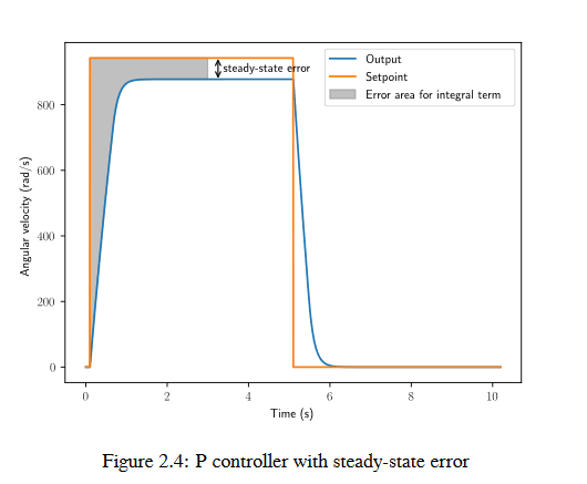
A common way of eliminating steady-state error is to integrate the error and add it to the control input. This increases the control effort until the system converges. Figure 2.4 shows an example of steady-state error for a flywheel, and figure 2.5 shows how an integrator added to the flywheel controller eliminates it. However, too high of an integral gain can lead to overshoot, as shown in figure 2.6.
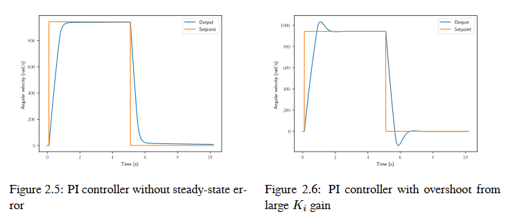
PID Controller Definition
Note
For information on using the WPILib provided PIDController, see the relevant article.
When these terms are combined, one gets the typical definition for a PID controller.
where \(K_p\) is the proportional gain, \(K_i\) is the integral gain, \(K_d\) is the derivative gain, \(e(t)\) is the error at the current time \(t\), and \(\tau\) is the integration variable.
The below figure shows a block diagram for a PID controller.
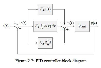
Response Types
A system driven by a PID controller generally has three types of responses: underdamped, over-damped, and critically damped. These are shown in figure 2.8.
For the step responses in figure 2.7, rise time is the time the system takes to initially reach the reference after applying the step input. Settling time is the time the system takes to settle at the reference after the step input is applied.
An underdamped response oscillates around the reference before settling. An overdamped response
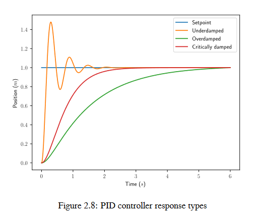
is slow to rise and does not overshoot the reference. A critically damped response has the fastest rise time without overshooting the reference.
Tuning a PID Controller
These steps apply to position PID controllers. Velocity PID controllers typically don’t need \(K_d\).
Set \(K_p\), \(K_i\), and \(K_d\) to zero.
Increase \(K_p\) until the output starts to oscillate around the setpoint.
Increase \(K_d\) as much as possible without introducing jittering in the system response.
Plot the position setpoint, velocity setpoint, measured position, and measured velocity. The velocity setpoint can be obtained via numerical differentiation of the position setpoint (i.e., \(v_{desired,k} = \frac{r_k - r_{k-1}}{\Delta t}\)). Increase \(K_p\) until the position tracks well, then increase \(K_d\) until the velocity tracks well.
If the controller settles at an output above or below the setpoint, one can increase \(K_i\) such that the controller reaches the setpoint in a reasonable amount of time. However, a steady-state feedforward is strongly preferred over integral control (especially for PID control).
Important
Adding an integral gain to the controller is an incorrect way to eliminate steady-state error. A better approach would be to tune it with an integrator added to the plant, but this requires a model. Since we are doing output-based rather than model-based control, our only option is to add an integrator to the controller.
Beware that if \(K_i\) is too large, integral windup can occur. Following a large change in setpoint, the integral term can accumulate an error larger than the maximal control input. As a result, the system overshoots and continues to increase until this accumulated error is unwound.
Note
The frc-characterization toolsuite can be used to model your system and give accurate Proportional and Derivative values. This is preferred over tuning the controller yourself.
Actuator Saturation
A controller calculates its output based on the error between the reference and the current state. Plant in the real world don’t have unlimited control authority available for the controller to apply. When the actuator limits are reached, the controller acts as if the gain has been temporarily reduced.
We’ll try to explain this through a bit of math. Let’s say we have a controller \(u = k(r - x)\) where \(u\) is the control effort, \(k\) is the gain, \(r\) is the reference, and \(x\) is the current state. Let \(u_{max}\) be the limit of the actuator’s output which is less than the uncapped value of \(u\) and \(k_{max}\) be the associated maximum gain. We will now compare the capped and uncapped controllers for the same reference and current state.
For the inequality to hold, \(k_{max}\) must be less than the original value for \(k\). This reduced gain is evident in a system response when there is a linear change in state instead of an exponential one as it approaches the reference. This is due to the control effort no longer following a decaying exponential plot. Once the system is closer to the reference, the controller will stop saturating and produce realistic controller values again.
Filters
Note
The data used to generate the various demonstration plots in this section can be found here.
This section describes a number of filters included with WPILib that are useful for noise reduction and/or input smoothing.
Introduction to Filters
Filters are some of the most common tools used in modern technology, and find numerous applications in robotics in both signal processing and controls. Understanding the notion of a filter is crucial to understanding the utility of the various types of filters provided by WPILib.
What Is a Filter?
Note
For the sake of this article, we will assume all data are single-dimensional time-series data. Obviously, the concepts involved are more general than this - but a full/rigorous discussion of signals and filtering is out of the scope of this documentation.
So, what exactly is a filter, then? Simply put, a filter is a mapping from a stream of inputs to a stream of outputs. That is to say, the value output by a filter (in principle) can depend not only on the current value of the input, but on the entire set of past and future values (of course, in practice, the filters provided by WPILib are implementable in real-time on streaming data; accordingly, they can only depend on the past values of the input, and not on future values). This is an important concept, because generally we use filters to remove/mitigate unwanted dynamics from a signal. When we filter a signal, we’re interested in modifying how the signal changes over time.
Effects of Using a Filter
Noise Reduction
One of the most typical uses of a filter is for noise reduction. A filter that reduces noise is called a low-pass filter (because it allows low frequencies to “pass through,” while blocking high-frequencies). Most of the filters currently included in WPILib are effectively low-pass filters.
Rate Limiting
Filters are also commonly used to reduce the rate at which a signal can change. This is closely related to noise reduction, and filters that reduce noise also tend to limit the rate of change of their output.
Edge Detection
The counterpart to the low-pass filter is the high-pass filter, which only permits high frequencies to pass through to the output. High-pass filters can be somewhat tricky to build intuition for, but a common usage for a high-pass filter is edge-detection - since high-pass filters will reflect sudden changes in the input while ignoring slower changes, they are useful for determining the location of sharp discontinuities in the signal.
Phase Lag
An unavoidable negative effect of a real-time low-pass filter is the introduction of “phase lag.” Since, as mentioned earlier, a real-time filter can only depend on past values of the signal (we cannot time-travel to obtain the future values), the filtered value takes some time to “catch up” when the input starts changing. The greater the noise-reduction, the greater the introduced delay. This is, in many ways, the fundamental trade-off of real-time filtering, and should be the primary driving factor of your filter design.
Interestingly, high-pass filters introduce a phase lead, as opposed to a phase lag, as they exacerbate local changes to the value of the input.
Linear Filters
The first (and most commonly-employed) sort of filter that WPILib supports is a linear filter - or, more specifically, a linear time-invariant (LTI) filter.
An LTI filter is, put simply, a weighted moving average - the value of the output stream at any given time is a localized, weighted average of the inputs near that time. The difference between different types of LTI filters is thus reducible to the difference in the choice of the weighting function (also known as a “window function” or an “impulse response”) used. Mathematically, this kind of moving average is known as a convolution.
There are two broad “sorts” of impulse responses: infinite impulse responses (IIR), and finite impulse responses (FIR).
Infinite impulse responses have infinite “support” - that is, they are nonzero over an infinitely-large region. This means, broadly, that they also have infinite “memory” - once a value appears in the input stream, it will influence all subsequent outputs, forever. This is typically undesirable from a strict signal-processing perspective, however filters with infinite impulse responses tend to be very easy to compute as they can be expressed by simple recursion relations.
Finite impulse responses have finite “support” - that is, they are nonzero on a bounded region. The “archetypical” FIR filter is a flat moving average - that is, simply setting the output equal to the average of the past n inputs. FIR filters tend to have more-desirable properties than IIR filters, but are more costly to compute.
Linear filters are supported in WPILib through the LinearFilter class (Java, C++).
Creating a LinearFilter
Note
The C++ LinearFilter class is templated on the data type used for the input.
Note
Because filters have “memory”, each input stream requires its own filter object. Do not attempt to use the same filter object for multiple input streams.
While it is possible to directly instantiate LinearFilter class to build a custom filter, it is far more convenient (and common) to use one of the supplied factory methods, instead:
singlePoleIIR
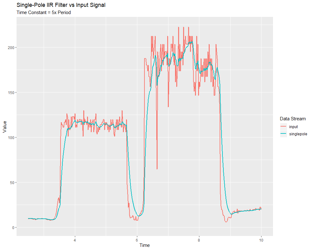
The singlePoleIIR() factory method creates a single-pole infinite impulse response filter (also known as exponential smoothing, on account of having an exponential impulse response). This is the “go-to,” “first-try” low-pass filter in most applications; it is computationally trivial and works in most cases.
// Creates a new Single-Pole IIR filter
// Time constant is 0.1 seconds
// Period is 0.02 seconds - this is the standard FRC main loop period
LinearFilter filter = LinearFilter.singlePoleIIR(0.1, 0.02);
// Creates a new Single-Pole IIR filter
// Time constant is 0.1 seconds
// Period is 0.02 seconds - this is the standard FRC main loop period
frc::LinearFilter<double> filter = frc::LinearFilter<double>::SinglePoleIIR(0.1_s, 0.02_s);
The “time constant” parameter determines the “characteristic timescale” of the filter’s impulse response; the filter will cancel out any signal dynamics that occur on timescales significantly shorter than this. Relatedly, it is also the approximate timescale of the introduced phase lag. The reciprocal of this timescale, multiplied by 2 pi, is the “cutoff frequency” of the filter.
The “period” parameter is the period at which the filter’s calculate() method will be called. For the vast majority of implementations, this will be the standard main robot loop period of 0.02 seconds.
movingAverage
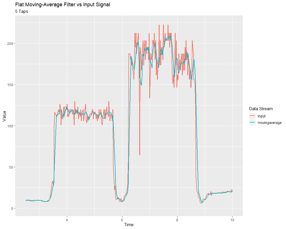
The movingAverage factory method creates a simple flat moving average filter. This is the simplest possible low-pass FIR filter, and is useful in many of the same contexts as the single-pole IIR filter. It is somewhat more costly to compute, but generally behaves in a somewhat nicer manner.
// Creates a new flat moving average filter
// Average will be taken over the last 5 samples
LinearFilter filter = LinearFilter.movingAverage(5);
// Creates a new flat moving average filter
// Average will be taken over the last 5 samples
frc::LinearFilter<double> filter = frc::LinearFilter<double>::MovingAverage(5);
The “taps” parameter is the number of samples that will be included in the flat moving average. This behaves similarly to the “time constant” above - the effective time constant is the number of taps times the period at which calculate() is called.
highPass
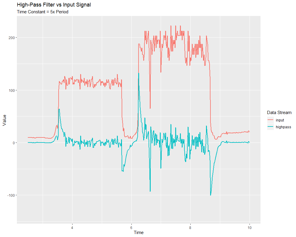
The highPass factory method creates a simple first-order infinite impulse response high-pass filter. This is the “counterpart” to the singlePoleIIR.
// Creates a new high-pass IIR filter
// Time constant is 0.1 seconds
// Period is 0.02 seconds - this is the standard FRC main loop period
LinearFilter filter = LinearFilter.highPass(0.1, 0.02);
// Creates a new high-pass IIR filter
// Time constant is 0.1 seconds
// Period is 0.02 seconds - this is the standard FRC main loop period
frc::LinearFilter<double> filter = frc::LinearFilter<double>::HighPass(0.1_s, 0.02_s);
The “time constant” parameter determines the “characteristic timescale” of the filter’s impulse response; the filter will cancel out any signal dynamics that occur on timescales significantly longer than this. Relatedly, it is also the approximate timescale of the introduced phase lead. The reciprocal of this timescale, multiplied by 2 pi, is the “cutoff frequency” of the filter.
The “period” parameter is the period at which the filter’s calculate() method will be called. For the vast majority of implementations, this will be the standard main robot loop period of 0.02 seconds.
Using a LinearFilter
Note
In order for the created filter to obey the specified timescale parameter, its calculate() function must be called regularly at the specified period. If, for some reason, a significant lapse in calculate() calls must occur, the filter’s reset() method should be called before further use.
Once your filter has been created, using it is easy - simply call the calculate() method with the most recent input to obtain the filtered output:
// Calculates the next value of the output
filter.calculate(input);
// Calculates the next value of the output
filter.Calculate(input);
Median Filter
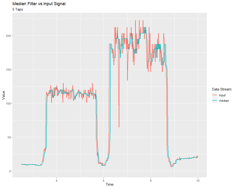
A robust alternative to the moving-average filter is the median filter. Where a moving average filter takes the arithmetic mean of the input over a moving sample window, a median filter (per the name) takes a median instead.
The median filter is most-useful for removing occasional outliers from an input stream. This makes it particularly well-suited to filtering inputs from distance sensors, which are prone to occasional interference. Unlike a moving average, the median filter will remain completely unaffected by small numbers of outliers, no matter how extreme.
The median filter is supported in WPILib through the MedianFilter class (Java, C++).
Creating a MedianFilter
Note
The C++ MedianFilter class is templated on the data type used for the input.
Note
Because filters have “memory”, each input stream requires its own filter object. Do not attempt to use the same filter object for multiple input streams.
Creating a MedianFilter is simple:
// Creates a MedianFilter with a window size of 5 samples
MedianFilter filter = new MedianFilter(5);
// Creates a MedianFilter with a window size of 5 samples
frc::MedianFilter<double> filter(5);
Using a MedianFilter
Once your filter has been created, using it is easy - simply call the calculate() method with the most recent input to obtain the filtered output:
// Calculates the next value of the output
filter.calculate(input);
// Calculates the next value of the output
filter.Calculate(input);
Slew Rate Limiter
A common use for filters in FRC® is to soften the behavior of control inputs (for example, the joystick inputs from your driver controls). Unfortunately, a simple low-pass filter is poorly-suited for this job; while a low-pass filter will soften the response of an input stream to sudden changes, it will also wash out fine control detail and introduce phase lag. A better solution is to limit the rate-of-change of the control input directly. This is performed with a slew rate limiter - a filter that caps the maximum rate-of-change of the signal.
A slew rate limiter can be thought of as a sort of primitive motion profile. In fact, the slew rate limiter is the first-order equivalent of the Trapezoidal Motion Profile supported by WPILib - it is precisely the limiting case of trapezoidal motion when the acceleration constraint is allowed to tend to infinity. Accordingly, the slew rate limiter is a good choice for applying a de-facto motion profile to a stream of velocity setpoints (or voltages, which are usually approximately proportional to velocity). For input streams that control positions, it is usually better to use a proper trapezoidal profile.
Slew rate limiting is supported in WPILib through the SlewRateLimiter class (Java, C++).
Creating a SlewRateLimiter
Note
The C++ SlewRateLimiter class is templated on the unit type of the input. For more information on C++ units, see The C++ Units Library.
Note
Because filters have “memory”, each input stream requires its own filter object. Do not attempt to use the same filter object for multiple input streams.
Creating a SlewRateLimiter is simple:
// Creates a SlewRateLimiter that limits the rate of change of the signal to 0.5 units per second
SlewRateLimiter filter = new SlewRateLimiter(0.5);
// Creates a SlewRateLimiter that limits the rate of change of the signal to 0.5 volts per second
frc::SlewRateLimiter<units::volts> filter{0.5_V / 1_s};
Using a SlewRateLimiter
Once your filter has been created, using it is easy - simply call the calculate() method with the most recent input to obtain the filtered output:
// Calculates the next value of the output
filter.calculate(input);
// Calculates the next value of the output
filter.Calculate(input);
Using a SlewRateLimiter with DifferentialDrive
Note
In the C++ example below, the filter is templated on double, rather than on a unit type, since joystick values are typically dimensionless.
A typical use of a SlewRateLimiter is to limit the acceleration of a robot’s drive. This can be especially handy for robots that are very top-heavy, or that have very powerful drives. To do this, apply a SlewRateLimiter to a value passed into your robot drive function:
// Ordinary call with no ramping applied
drivetrain.arcadeDrive(forward, turn);
// Slew-rate limits the forward/backward input, limiting forward/backward acceleration
drivetrain.arcadeDrive(filter.calculate(forward), turn);
// Ordinary call with no ramping applied
drivetrain.ArcadeDrive(forward, turn);
// Slew-rate limits the forward/backward input, limiting forward/backward acceleration
drivetrain.ArcadeDrive(filter.Calculate(forward), turn);
Debouncer
A debouncer is a filter used to eliminate unwanted quick on/off cycles (termed “bounces,” originally from the physical vibrations of a switch as it is thrown). These cycles are usually due to a sensor error like noise or reflections and not the actual event the sensor is trying to record.
Debouncing is implemented in WPILib by the Debouncer class (Java, C++), which filters a boolean stream so that the output only changes if the input sustains a change for some nominal time period.
Modes
The WPILib Debouncer can be configured in three different modes:
Rising (default): Debounces rising edges (transitions from false to true) only.
Falling: Debounces falling edges (transitions from true to false) only.
Both: Debounces all transitions.
Usage
// Initializes a DigitalInput on DIO 0
DigitalInput input = new DigitalInput(0);
// Creates a Debouncer in "both" mode.
Debouncer m_debouncer = new Debouncer(0.1, Debouncer.DebounceType.kBoth);
// So if currently false the signal must go true for at least .1 seconds before being read as a True signal.
if (m_debouncer.calculate(input.get())) {
// Do something now that the DI is True.
}
// Initializes a DigitalInput on DIO 0
frc::DigitalInput input{0};
// Creates a Debouncer in "both" mode.
frc::Debouncer m_debouncer{100_ms, frc::Debouncer::DebounceType::kBoth};
// So if currently false the signal must go true for at least .1 seconds before being read as a True signal.
if (m_debouncer.calculate(input.Get())) {
// Do something now that the DI is True.
}
Geometry Classes
This section covers the geometry classes of WPILib.
Coordinate Systems
In FRC®, there are two main coordinate systems that we use for representing objects’ positions.
Field Coordinate System
The field coordinate system (or global coordinate system) is an absolute coordinate system where a point on the field is designated as the origin. Positive \(\theta\) (theta) is in the counter-clockwise direction, and the positive x-axis points away from your alliance’s driver station wall, and the positive y-axis is perpendicular and to the left of the positive x-axis.

Note
The axes are shown at the middle of the field for visibility. The origins of the coordinate system for each alliance are shown below.
Below is an example of a field coordinate system overlayed on the 2020 FRC field. The red axes shown are for the red alliance, and the blue axes shown are for the blue alliance.
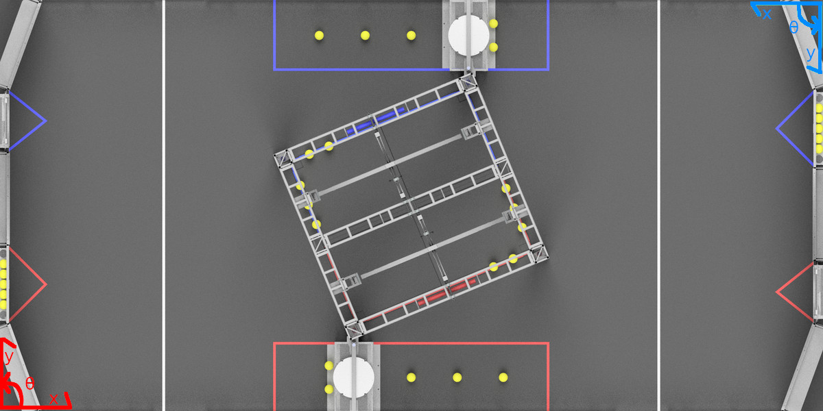
Robot Coordinate System
The robot coordinate system (or local coordinate system) is a relative coordinate system where the robot is the origin. The direction the robot is facing is the positive x axis, and the positive y axis is perpendicular, to the left of the robot. Positive \(\theta\) is counter-clockwise.
Note
WPILib’s Gyro class is clockwise-positive, so you have to invert the reading in order to get the rotation with either coordinate system.

Translation, Rotation, and Pose
Translation
Translation in 2 dimensions is represented by WPILib’s Translation2d class (Java, C++). This class has an x and y component, representing the point \((x, y)\) or the vector \(\begin{bmatrix}x \\ y \end{bmatrix}\) on a 2-dimensional coordinate system.
You can get the distance to another Translation2d object by using the getDistance(Translation2d other), which returns the distance to another Translation2d by using the Pythagorean theorem.
Note
Translation2d uses the C++ Units library. If you’re planning on using other WPILib classes that use Translation2d in Java, such as the trajectory generator, make sure to use meters.
Rotation
Rotation in 2 dimensions is representated by WPILib’s Rotation2d class (Java, C++). This class has an angle component, which represents the robot’s rotation relative to an axis on a 2-dimensional coordinate system. Positive rotations are counterclockwise.
Note
Rotation2d uses the C++ Units library. The contructor in Java accepts either the angle in radians, or the sine and cosine of the angle, but the fromDegrees method will construct a Rotation2d object from degrees.
Pose
Pose is a combination of both translation and rotation and is represented by the Pose2d class (Java, C++). It can be used to describe the pose of your robot in the field coordinate system, or the pose of objects, such as vision targets, relative to your robot in the robot coordinate system. Pose2d can also represent the vector \(\begin{bmatrix}x \\ y \\ \theta\end{bmatrix}\).
Transformations
Translation2d
Operations on a Translation2d perform operations to the vector represented by the Translation2d.
Addition: Addition between two
Translation2da and b can be performed usingplusin Java, or the+operator in C++. Addition adds the two vectors.Subtraction: Subtraction between two
Translation2dcan be performed usingminusin Java, or the binary-operator in C++. Subtraction subtracts the two vectors.Multiplication: Multiplication of a
Translation2dand a scalar can be performed usingtimesin Java, or the*operator in C++. This multiplies the vector by the scalar.Division: Division of a
Translation2dand a scalar can be performed usingdivin Java, or the/operator in C++. This divides the vector by the scalar.Rotation: Rotation of a
Translation2dby a counter-clockwise rotation \(\theta\) about the origin can be performed by usingrotateBy. This is equivalent to multiplying the vector by the matrix \(\begin{bmatrix} cos\theta & -sin\theta \\ sin\theta & cos\theta \end{bmatrix}\)Additionally, you can rotate a
Translation2dby 180 degrees by usingunaryMinusin Java, or the unary-operator in C++.
Rotation2d
Transformations for Rotation2d are just arithmetic operations on the angle measure represented by the Rotation2d.
plus(Java) or+(C++): Adds the rotation component ofotherto thisRotation2d’s rotation componentminus(Java) or binary-(C++): Subtracts the rotation component ofotherto thisRotation2d’s rotation componentunaryMinus(Java) or unary-(C++): Multiplies the rotation component by a scalar of -1.times(Java) or*(C++) : Multiplies the rotation component by a scalar.
Transform2d and Twist2d
WPILib provides 2 classes, Transform2d (Java, C++), which represents a transformation to a pose, and Twist2d (Java, C++) which represents a movement along an arc. Transform2d and Twist2d all have x, y and \(\theta\) components.
Transform2d represents a relative transformation. It has an translation and a rotation component. Transforming a Pose2d by a Transform2d rotates the translation component of the transform by the rotation of the pose, and then adds the rotated translation component and the rotation component to the pose. In other words, Pose2d.plus(Transform2d) returns \(\begin{bmatrix} x_p \\ y_p \\ \theta_p \end{bmatrix}+\begin{bmatrix} cos\theta_p & -sin\theta_p & 0 \\ sin\theta_p & cos\theta_p & 0 \\ 0 & 0 & 1 \end{bmatrix}\begin{bmatrix}x_t \\ y_t \\ \theta_t \end{bmatrix}\)
Twist2d represents a change in distance along an arc. Usually, this class is used to represent the movement of a drivetrain, where the x component is the forward distance driven, the y component is the distance driven to the side (left positive), and the \(\theta\) component is the change in heading. The underlying math behind finding the pose exponential (new pose after moving the pose forward along the curvature of the twist) can be found here in chapter 10.
Note
For nonholonomic drivetrains, the y component of a Twist2d should always be 0.
Both classes can be used to estimate robot location. Twist2d is used in WPILib’s odometry classes to update the robot’s pose based on movement, while Transform2d can be used to estimate the robot’s global position from vision data.
Controllers
This section describes various WPILib feedback and feedforward controller classes that are useful for controlling the motion of robot mechanisms, as well as motion-profiling classes that can automatically generate setpoints for use with these controllers.
PID Control in WPILib
Note
This article covers the in-code implementation of PID Control with WPILib’s provided library classes. Documentation describing the involved concepts in more detail is forthcoming.
Note
For a guide on implementing PID control through the command-based framework, see PID Control through PIDSubsystems and PIDCommands.
WPILib supports PID control of mechanisms through the PIDController class (Java, C++). This class handles the feedback loop calculation for the user, as well as offering methods for returning the error, setting tolerances, and checking if the control loop has reached its setpoint within the specified tolerances.
Using the PIDController Class
Note
The PIDController class in the frc namespace is deprecated - C++ teams should use the one in the frc2 namespace, instead. Likewise, Java teams should use the class in the wpilibj.controller package.
Constructing a PIDController
Note
While PIDController may be used asynchronously, it does not provide any thread safety features - ensuring threadsafe operation is left entirely to the user, and thus asynchronous usage is recommended only for advanced teams.
In order to use WPILib’s PID control functionality, users must first construct a PIDController object with the desired gains:
// Creates a PIDController with gains kP, kI, and kD
PIDController pid = new PIDController(kP, kI, kD);
// Creates a PIDController with gains kP, kI, and kD
frc2::PIDController pid{kP, kI, kD};
An optional fourth parameter can be provided to the constructor, specifying the period at which the controller will be run. The PIDController object is intended primarily for synchronous use from the main robot loop, and so this value is defaulted to 20ms.
Using the Feedback Loop Output
Note
The PIDController assumes that the calculate() method is being called regularly at an interval consistent with the configured period. Failure to do this will result in unintended loop behavior.
Warning
Unlike the old PIDController, the new PIDController does not automatically control an output from its own thread - users are required to call calculate() and use the resulting output in their own code.
Using the constructed PIDController is simple: simply call the calculate() method from the robot’s main loop (e.g. the robot’s autonomousPeriodic() method):
// Calculates the output of the PID algorithm based on the sensor reading
// and sends it to a motor
motor.set(pid.calculate(encoder.getDistance(), setpoint));
// Calculates the output of the PID algorithm based on the sensor reading
// and sends it to a motor
motor.Set(pid.Calculate(encoder.GetDistance(), setpoint));
Checking Errors
Note
getPositionError() and getVelocityError() are named assuming that the loop is controlling a position - for a loop that is controlling a velocity, these return the velocity error and the acceleration error, respectively.
The current error of the measured process variable is returned by the getPositionError() function, while its derivative is returned by the getVelocityError() function:
Specifying and Checking Tolerances
Note
If only a position tolerance is specified, the velocity tolerance defaults to infinity.
Note
As above, “position” refers to the process variable measurement, and “velocity” to its derivative - thus, for a velocity loop, these are actually velocity and acceleration, respectively.
Occasionally, it is useful to know if a controller has tracked the setpoint to within a given tolerance - for example, to determine if a command should be ended, or (while following a motion profile) if motion is being impeded and needs to be re-planned.
To do this, we first must specify the tolerances with the setTolerance() method; then, we can check it with the atSetpoint() method.
// Sets the error tolerance to 5, and the error derivative tolerance to 10 per second
pid.setTolerance(5, 10);
// Returns true if the error is less than 5 units, and the
// error derivative is less than 10 units
pid.atSetpoint();
// Sets the error tolerance to 5, and the error derivative tolerance to 10 per second
pid.SetTolerance(5, 10);
// Returns true if the error is less than 5 units, and the
// error derivative is less than 10 units
pid.AtSetpoint();
Resetting the Controller
It is sometimes desirable to clear the internal state (most importantly, the integral accumulator) of a PIDController, as it may be no longer valid (e.g. when the PIDController has been disabled and then re-enabled). This can be accomplished by calling the reset() method.
Setting a Max Integrator Value
Note
Integrators introduce instability and hysteresis into feedback loop systems. It is strongly recommended that teams avoid using integral gain unless absolutely no other solution will do - very often, problems that can be solved with an integrator can be better solved through use of a more-accurate feedforward.
A typical problem encountered when using integral feedback is excessive “wind-up” causing the system to wildly overshoot the setpoint. This can be alleviated in a number of ways - the WPILib PIDController class enforces an integrator range limiter to help teams overcome this issue.
By default, the total output contribution from the integral gain is limited to be between -1.0 and 1.0.
The range limits may be increased or decreased using the setIntegratorRange() method.
// The integral gain term will never add or subtract more than 0.5 from
// the total loop output
pid.setIntegratorRange(-0.5, 0.5);
// The integral gain term will never add or subtract more than 0.5 from
// the total loop output
pid.SetIntegratorRange(-0.5, 0.5);
Setting Continuous Input
Warning
If your mechanism is not capable of fully continuous rotational motion (e.g. a turret without a slip ring, whose wires twist as it rotates), do not enable continuous input unless you have implemented an additional safety feature to prevent the mechanism from moving past its limit!
Warning
The continuous input function does not automatically wrap your input values - be sure that your input values, when using this feature, are never outside of the specified range!
Some process variables (such as the angle of a turret) are measured on a circular scale, rather than a linear one - that is, each “end” of the process variable range corresponds to the same point in reality (e.g. 360 degrees and 0 degrees). In such a configuration, there are two possible values for any given error, corresponding to which way around the circle the error is measured. It is usually best to use the smaller of these errrors.
To configure a PIDController to automatically do this, use the enableContinuousInput() method:
// Enables continuous input on a range from -180 to 180
pid.enableContinuousInput(-180, 180);
// Enables continuous input on a range from -180 to 180
pid.EnableContinuousInput(-180, 180);
Clamping Controller Output
Unlike the old PIDController, the new controller does not offer any output clamping features, as the user is expected to use the loop output themselves. Output clamping can be easily achieved by composing the controller with WPI’s clamp() function (or std::clamp in c++):
// Clamps the controller output to between -0.5 and 0.5
MathUtil.clamp(pid.calculate(encoder.getDistance(), setpoint), -0.5, 0.5);
// Clamps the controller output to between -0.5 and 0.5
std::clamp(pid.Calculate(encoder.GetDistance(), setpoint), -0.5, 0.5);
Feedforward Control in WPILib
So far, we’ve used feedback control for reference tracking (making a system’s output follow a desired reference signal). While this is effective, it’s a reactionary measure; the system won’t start applying control effort until the system is already behind. If we could tell the controller about the desired movement and required input beforehand, the system could react quicker and the feedback controller could do less work. A controller that feeds information forward into the plant like this is called a feedforward controller.
A feedforward controller injects information about the system’s dynamics (like a mathematical model does) or the intended movement. Feedforward handles parts of the control actions we already know must be applied to make a system track a reference, then feedback compensates for what we do not or cannot know about the system’s behavior at runtime.
There are two types of feedforwards: model-based feedforward and feedforward for unmodeled dynamics. The first solves a mathematical model of the system for the inputs required to meet desired velocities and accelerations. The second compensates for unmodeled forces or behaviors directly so the feedback controller doesn’t have to. Both types can facilitate simpler feedback controllers. We’ll cover several examples below.
Note
The WPILib feedforward classes closely match the available mechanism characterization tools available in the frc-characterization toolsuite - the characterization toolsuite can be used to quickly and effectively determine the correct gains for each type of feedforward. The toolsuite will indicate the appropriate units for each of the gains.
WPILib provides a number of classes to help users implement accurate feedforward control for their mechanisms. In many ways, an accurate feedforward is more important than feedback to effective control of a mechanism. Since most FRC® mechanisms closely obey well-understood system equations, starting with an accurate feedforward is both easy and hugely beneficial to accurate and robust mechanism control.
WPILib currently provides the following three helper classes for feedforward control:
SimpleMotorFeedforward
Note
In C++, the SimpleMotorFeedforward class is templated on the unit type used for distance measurements, which may be angular or linear. The passed-in gains must have units consistent with the distance units, or a compile-time error will be thrown. kS should have units of volts, kV should have units of volts * seconds / distance, and kA should have units of volts * seconds^2 / distance. For more information on C++ units, see The C++ Units Library.
Note
The Java feedforward components will calculate outputs in units determined by the units of the user-provided feedforward gains. Users must take care to keep units consistent, as WPILibJ does not have a type-safe unit system.
The SimpleMotorFeedforward class calculates feedforwards for mechanisms that consist of permanent-magnet DC motors with no external loading other than friction and inertia, such as flywheels and robot drives.
To create a SimpleMotorFeedforward, simply construct it with the required gains:
Note
The kA gain can be omitted, and if it is, will default to a value of zero. For many mechanisms, especially those with little inertia, it is not necessary.
// Create a new SimpleMotorFeedforward with gains kS, kV, and kA
SimpleMotorFeedforward feedforward = new SimpleMotorFeedforward(kS, kV, kA);
// Create a new SimpleMotorFeedforward with gains kS, kV, and kA
// Distance is measured in meters
frc::SimpleMotorFeedforward<units::meters> feedforward(kS, kV, kA);
To calculate the feedforward, simply call the calculate() method with the desired motor velocity and acceleration:
Note
The acceleration argument may be omitted from the calculate() call, and if it is, will default to a value of zero. This should be done whenever there is not a clearly-defined acceleration setpoint.
// Calculates the feedforward for a velocity of 10 units/second and an acceleration of 20 units/second^2
// Units are determined by the units of the gains passed in at construction.
feedforward.calculate(10, 20);
// Calculates the feedforward for a velocity of 10 meters/second and an acceleration of 20 meters/second^2
// Output is in volts
feedforward.Calculate(10_mps, 20_mps_sq);
ArmFeedforward
Note
In C++, the ArmFeedforward class assumes distances are angular, not linear. The passed-in gains must have units consistent with the angular unit, or a compile-time error will be thrown. kS and kCos should have units of volts, kV should have units of volts * seconds / radians, and kA should have units of volts * seconds^2 / radians. For more information on C++ units, see The C++ Units Library.
Note
The Java feedforward components will calculate outputs in units determined by the units of the user-provided feedforward gains. Users must take care to keep units consistent, as WPILibJ does not have a type-safe unit system.
The ArmFeedforward class calculates feedforwards for arms that are controlled directly by a permanent-magnet DC motor, with external loading of friction, inertia, and mass of the arm. This is an accurate model of most arms in FRC.
To create an ArmFeedforward, simply construct it with the required gains:
Note
The kA gain can be omitted, and if it is, will default to a value of zero. For many mechanisms, especially those with little inertia, it is not necessary.
// Create a new ArmFeedforward with gains kS, kCos, kV, and kA
ArmFeedforward feedforward = new ArmFeedforward(kS, kCos, kV, kA);
// Create a new ArmFeedforward with gains kS, kCos, kV, and kA
frc::ArmFeedforward feedforward(kS, kCos, kV, kA);
To calculate the feedforward, simply call the calculate() method with the desired arm position, velocity, and acceleration:
Note
The acceleration argument may be omitted from the calculate() call, and if it is, will default to a value of zero. This should be done whenever there is not a clearly-defined acceleration setpoint.
// Calculates the feedforward for a position of 1 units, a velocity of 2 units/second, and
// an acceleration of 3 units/second^2
// Units are determined by the units of the gains passed in at construction.
feedforward.calculate(1, 2, 3);
// Calculates the feedforward for a position of 1 radians, a velocity of 2 radians/second, and
// an acceleration of 3 radians/second^2
// Output is in volts
feedforward.Calculate(1_rad, 2_rad_per_s, 3_rad/(1_s * 1_s));
ElevatorFeedforward
Note
In C++, the ElevatorFeedforward class is templated on the unit type used for distance measurements, which may be angular or linear. The passed-in gains must have units consistent with the distance units, or a compile-time error will be thrown. kS and kG should have units of volts, kV should have units of volts * seconds / distance, and kA should have units of volts * seconds^2 / distance. For more information on C++ units, see The C++ Units Library.
Note
The Java feedforward components will calculate outputs in units determined by the units of the user-provided feedforward gains. Users must take care to keep units consistent, as WPILibJ does not have a type-safe unit system.
The ElevatorFeedforward class calculates feedforwards for elevators that consist of permanent-magnet DC motors loaded by friction, inertia, and the mass of the elevator. This is an accurate model of most elevators in FRC.
To create a ElevatorFeedforward, simply construct it with the required gains:
Note
The kA gain can be omitted, and if it is, will default to a value of zero. For many mechanisms, especially those with little inertia, it is not necessary.
// Create a new ElevatorFeedforward with gains kS, kG, kV, and kA
ElevatorFeedforward feedforward = new ElevatorFeedforward(kS, kG, kV, kA);
// Create a new ElevatorFeedforward with gains kS, kV, and kA
// Distance is measured in meters
frc::ElevatorFeedforward<units::meters> feedforward(kS, kG, kV, kA);
To calculate the feedforward, simply call the calculate() method with the desired motor velocity and acceleration:
Note
The acceleration argument may be omitted from the calculate() call, and if it is, will default to a value of zero. This should be done whenever there is not a clearly-defined acceleration setpoint.
// Calculates the feedforward for a position of 10 units, velocity of 20 units/second,
// and an acceleration of 30 units/second^2
// Units are determined by the units of the gains passed in at construction.
feedforward.calculate(10, 20, 30);
// Calculates the feedforward for a position of 10 meters, velocity of 20 meters/second,
// and an acceleration of 30 meters/second^2
// Output is in volts
feedforward.Calculate(10_m, 20_mps, 30_mps_sq);
Using Feedforward to Control Mechanisms
Note
Since feedforward voltages are physically meaningful, it is best to use the setVoltage() (Java, C++) method when applying them to motors to compensate for “voltage sag” from the battery.
Feedforward control can be used entirely on its own, without a feedback controller. This is known as “open-loop” control, and for many mechanisms (especially robot drives) can be perfectly satisfactory. A SimpleMotorFeedforward might be employed to control a robot drive as follows:
public void tankDriveWithFeedforward(double leftVelocity, double rightVelocity) {
leftMotor.setVoltage(feedforward.calculate(leftVelocity));
rightMotor.setVoltage(feedForward.calculate(rightVelocity));
}
void TankDriveWithFeedforward(units::meters_per_second_t leftVelocity,
units::meters_per_second_t rightVelocity) {
leftMotor.SetVoltage(feedforward.Calculate(leftVelocity));
rightMotor.SetVoltage(feedforward.Calculate(rightVelocity));
}
Combining Feedforward and PID Control
Note
This article covers the in-code implementation of combined feedforward/PID control with WPILib’s provided library classes. Documentation describing the involved concepts in more detail is forthcoming.
Feedforward and feedback controllers can each be used in isolation, but are most effective when combined together. Thankfully, combining these two control methods is exceedingly straightforward - one simply adds their outputs together.
Using Feedforward with a PIDController
Users familiar with the old PIDController class may notice the lack of any feedforward gain in the new controller. As users are expected to use the controller output themselves, there is no longer any need for the PIDController to implement feedforward - users may simply add any feedforward they like to the output of the controller before sending it to their motors:
// Adds a feedforward to the loop output before sending it to the motor
motor.setVoltage(pid.calculate(encoder.getDistance(), setpoint) + feedforward);
// Adds a feedforward to the loop output before sending it to the motor
motor.SetVoltage(pid.Calculate(encoder.GetDistance(), setpoint) + feedforward);
Moreover, feedforward is a separate feature entirely from feedback, and thus has no reason to be handled in the same controller object, as this violates separation of concerns. WPILib comes with several helper classes to compute accurate feedforward voltages for common FRC® mechanisms - for more information, see Feedforward Control in WPILib.
Using Feedforward Components with PID
Note
Since feedforward voltages are physically meaningful, it is best to use the setVoltage() (Java, C++) method when applying them to motors to compensate for “voltage sag” from the battery.
What might a more complete example of combined feedforward/PID control look like? Consider the drive example from the feedforward page. We can easily modify this to include feedback control (with a SimpleMotorFeedforward component):
public void tankDriveWithFeedforwardPID(double leftVelocitySetpoint, double rightVelocitySetpoint) {
leftMotor.setVoltage(feedforward.calculate(leftVelocitySetpoint)
+ leftPID.calculate(leftEncoder.getRate(), leftVelocitySetpoint);
rightMotor.setVoltage(feedForward.calculate(rightVelocitySetpoint)
+ rightPID.calculate(rightEncoder.getRate(), rightVelocitySetpoint);
}
void TankDriveWithFeedforwardPID(units::meters_per_second_t leftVelocitySetpoint,
units::meters_per_second_t rightVelocitySetpoint) {
leftMotor.SetVoltage(feedforward.Calculate(leftVelocitySetpoint)
+ leftPID.Calculate(leftEncoder.getRate(), leftVelocitySetpoint.value());
rightMotor.SetVoltage(feedforward.Calculate(rightVelocitySetpoint)
+ rightPID.Calculate(rightEncoder.getRate(), rightVelocitySetpoint.value());
}
Other mechanism types can be handled similarly.
Trapezoidal Motion Profiles in WPILib
Note
This article covers the in-code generation of trapezoidal motion profiles. Documentation describing the involved concepts in more detail is forthcoming.
Note
For a guide on implementing the TrapezoidProfile class in the command-based framework framework, see Motion Profiling through TrapezoidProfileSubsystems and TrapezoidProfileCommands.
Note
The TrapezoidProfile class, used on its own, is most useful when composed with a custom controller (such as a “smart” motor controller with a built-in PID functionality). To integrate it with a WPILib PIDController, see Combining Motion Profiling and PID Control with ProfiledPIDController.
While feedforward and feedback control offer convenient ways to achieve a given setpoint, we are often still faced with the problem of generating setpoints for our mechanisms. While the naive approach of immediately commanding a mechanism to its desired state may work, it is often suboptimal. To improve the handling of our mechanisms, we often wish to command mechanisms to a sequence of setpoints that smoothly interpolate between its current state, and its desired goal state.
To help users do this, WPILib provides a TrapezoidProfile class (Java, C++).
Creating a TrapezoidProfile
Note
In C++, the TrapezoidProfile class is templated on the unit type used for distance measurements, which may be angular or linear. The passed-in values must have units consistent with the distance units, or a compile-time error will be thrown. For more information on C++ units, see The C++ Units Library.
Constraints
Note
The various feedforward helper classes provide methods for calculating the maximum simultaneously-achievable velocity and acceleration of a mechanism. These can be very useful for calculating appropriate motion constraints for your TrapezoidProfile.
In order to create a trapezoidal motion profile, we must first impose some constraints on the desired motion. Namely, we must specify a maximum velocity and acceleration that the mechanism will be expected to achieve during the motion. To do this, we create an instance of the TrapezoidProfile.Constraints class (Java, C++):
// Creates a new set of trapezoidal motion profile constraints
// Max velocity of 10 meters per second
// Max acceleration of 20 meters per second squared
new TrapezoidProfile.Constraints(10, 20);
// Creates a new set of trapezoidal motion profile constraints
// Max velocity of 10 meters per second
// Max acceleration of 20 meters per second squared
frc::TrapezoidProfile<units::meters>::Constraints{10_mps, 20_mps_sq};
Start and End States
Next, we must specify the desired starting and ending states for our mechanisms using the TrapezoidProfile.State class (Java, C++). Each state has a position and a velocity:
// Creates a new state with a position of 5 meters
// and a velocity of 0 meters per second
new TrapezoidProfile.State(5, 0);
// Creates a new state with a position of 5 meters
// and a velocity of 0 meters per second
frc::TrapezoidProfile<units::meters>::State{5_m, 0_mps};
Putting It All Together
Note
C++ is often able to infer the type of the inner classes, and thus a simple initializer list (without the class name) can be sent as a parameter. The full class names are included in the example below for clarity.
Now that we know how to create a set of constraints and the desired start/end states, we are ready to create our motion profile. The TrapezoidProfile constructor takes 3 parameters, in order: the constraints, the goal state, and the initial state.
// Creates a new TrapezoidProfile
// Profile will have a max vel of 5 meters per second
// Profile will have a max acceleration of 10 meters per second squared
// Profile will end stationary at 5 meters
// Profile will start stationary at zero position
TrapezoidProfile profile = new TrapezoidProfile(new TrapezoidProfile.Constraints(5, 10),
new TrapezoidProfile.State(5, 0),
new TrapezoidProfile.State(0, 0));
// Creates a new TrapezoidProfile
// Profile will have a max vel of 5 meters per second
// Profile will have a max acceleration of 10 meters per second squared
// Profile will end stationary at 5 meters
// Profile will start stationary at zero position
frc::TrapezoidProfile<units::meters> profile{
frc::TrapezoidProfile<units::meters>::Constraints{5_mps, 10_mps_sq},
frc::TrapezoidProfile<units::meters>::State{5_m, 0_mps},
frc::TrapezoidProfile<units::meters>::State{0_m, 0_mps}};
Using a TrapezoidProfile
Sampling the Profile
Once we’ve created a TrapezoidProfile, using it is very simple: to get the profile state at the given time after the profile has started, call the calculate() method:
// Returns the motion profile state after 5 seconds of motion
profile.calculate(5);
// Returns the motion profile state after 5 seconds of motion
profile.Calculate(5_s);
Using the State
The calculate method returns a TrapezoidProfile.State class (the same one that was used to specify the initial/end states when constructing the profile). To use this for actual control, simply pass the contained position and velocity values to whatever controller you wish (for example, a PIDController):
var setpoint = profile.calculate(elapsedTime);
controller.calculate(encoder.getDistance(), setpoint.position);
auto setpoint = profile.Calculate(elapsedTime);
controller.Calculate(encoder.GetDistance(), setpoint.position.value());
Complete Usage Example
Note
In this example, the profile is re-computed every timestep. This is a somewhat different usage technique than is detailed above, but works according to the same principles - the profile is sampled at at a time corresponding to the loop period to get the setpoint for the next loop iteration.
A more complete example of TrapezoidProfile usage is provided in the ElevatorTrapezoidProfile example project (Java, C++):
5package edu.wpi.first.wpilibj.examples.elevatortrapezoidprofile;
6
7import edu.wpi.first.math.controller.SimpleMotorFeedforward;
8import edu.wpi.first.math.trajectory.TrapezoidProfile;
9import edu.wpi.first.wpilibj.Joystick;
10import edu.wpi.first.wpilibj.TimedRobot;
11
12public class Robot extends TimedRobot {
13 private static double kDt = 0.02;
14
15 private final Joystick m_joystick = new Joystick(1);
16 private final ExampleSmartMotorController m_motor = new ExampleSmartMotorController(1);
17 // Note: These gains are fake, and will have to be tuned for your robot.
18 private final SimpleMotorFeedforward m_feedforward = new SimpleMotorFeedforward(1, 1.5);
19
20 private final TrapezoidProfile.Constraints m_constraints =
21 new TrapezoidProfile.Constraints(1.75, 0.75);
22 private TrapezoidProfile.State m_goal = new TrapezoidProfile.State();
23 private TrapezoidProfile.State m_setpoint = new TrapezoidProfile.State();
24
25 @Override
26 public void robotInit() {
27 // Note: These gains are fake, and will have to be tuned for your robot.
28 m_motor.setPID(1.3, 0.0, 0.7);
29 }
30
31 @Override
32 public void teleopPeriodic() {
33 if (m_joystick.getRawButtonPressed(2)) {
34 m_goal = new TrapezoidProfile.State(5, 0);
35 } else if (m_joystick.getRawButtonPressed(3)) {
36 m_goal = new TrapezoidProfile.State(0, 0);
37 }
38
39 // Create a motion profile with the given maximum velocity and maximum
40 // acceleration constraints for the next setpoint, the desired goal, and the
41 // current setpoint.
42 var profile = new TrapezoidProfile(m_constraints, m_goal, m_setpoint);
43
44 // Retrieve the profiled setpoint for the next timestep. This setpoint moves
45 // toward the goal while obeying the constraints.
46 m_setpoint = profile.calculate(kDt);
47
48 // Send setpoint to offboard controller PID
49 m_motor.setSetpoint(
50 ExampleSmartMotorController.PIDMode.kPosition,
51 m_setpoint.position,
52 m_feedforward.calculate(m_setpoint.velocity) / 12.0);
53 }
54}
5#include <frc/Joystick.h>
6#include <frc/TimedRobot.h>
7#include <frc/controller/SimpleMotorFeedforward.h>
8#include <frc/trajectory/TrapezoidProfile.h>
9#include <units/acceleration.h>
10#include <units/length.h>
11#include <units/time.h>
12#include <units/velocity.h>
13#include <units/voltage.h>
14#include <wpi/numbers>
15
16#include "ExampleSmartMotorController.h"
17
18class Robot : public frc::TimedRobot {
19 public:
20 static constexpr units::second_t kDt = 20_ms;
21
22 Robot() {
23 // Note: These gains are fake, and will have to be tuned for your robot.
24 m_motor.SetPID(1.3, 0.0, 0.7);
25 }
26
27 void TeleopPeriodic() override {
28 if (m_joystick.GetRawButtonPressed(2)) {
29 m_goal = {5_m, 0_mps};
30 } else if (m_joystick.GetRawButtonPressed(3)) {
31 m_goal = {0_m, 0_mps};
32 }
33
34 // Create a motion profile with the given maximum velocity and maximum
35 // acceleration constraints for the next setpoint, the desired goal, and the
36 // current setpoint.
37 frc::TrapezoidProfile<units::meters> profile{m_constraints, m_goal,
38 m_setpoint};
39
40 // Retrieve the profiled setpoint for the next timestep. This setpoint moves
41 // toward the goal while obeying the constraints.
42 m_setpoint = profile.Calculate(kDt);
43
44 // Send setpoint to offboard controller PID
45 m_motor.SetSetpoint(ExampleSmartMotorController::PIDMode::kPosition,
46 m_setpoint.position.value(),
47 m_feedforward.Calculate(m_setpoint.velocity) / 12_V);
48 }
49
50 private:
51 frc::Joystick m_joystick{1};
52 ExampleSmartMotorController m_motor{1};
53 frc::SimpleMotorFeedforward<units::meters> m_feedforward{
54 // Note: These gains are fake, and will have to be tuned for your robot.
55 1_V, 1.5_V * 1_s / 1_m};
56
57 frc::TrapezoidProfile<units::meters>::Constraints m_constraints{1.75_mps,
58 0.75_mps_sq};
59 frc::TrapezoidProfile<units::meters>::State m_goal;
60 frc::TrapezoidProfile<units::meters>::State m_setpoint;
61};
62
63#ifndef RUNNING_FRC_TESTS
64int main() {
65 return frc::StartRobot<Robot>();
66}
67#endif
Combining Motion Profiling and PID Control with ProfiledPIDController
Note
For a guide on implementing the ProfiledPIDController class in the command-based framework framework, see Combining Motion Profiling and PID in Command-Based.
In the previous article, we saw how to use the TrapezoidProfile class to create and use a trapezoidal motion profile. The example code from that article demonstrates manually composing the TrapezoidProfile class with the external PID control feature of a “smart” motor controller.
This combination of functionality (a motion profile for generating setpoints combined with a PID controller for following them) is extremely common. To facilitate this, WPILib comes with a ProfiledPIDController class (Java, C++) that does most of the work of combining these two functionalities. The API of the ProfiledPIDController is very similar to that of the PIDController, allowing users to add motion profiling to a PID-controlled mechanism with very few changes to their code.
Using the ProfiledPIDController class
Note
In C++, the ProfiledPIDController class is templated on the unit type used for distance measurements, which may be angular or linear. The passed-in values must have units consistent with the distance units, or a compile-time error will be thrown. For more information on C++ units, see The C++ Units Library.
Note
Much of the functionality of ProfiledPIDController is effectively identical to that of PIDController. Accordingly, this article will only cover features that are substantially-changed to accommodate the motion profiling functionality. For information on standard PIDController features, see PID Control in WPILib.
Constructing a ProfiledPIDController
Note
C++ is often able to infer the type of the inner classes, and thus a simple initializer list (without the class name) can be sent as a parameter. The full class name is included in the example below for clarity.
Creating a ProfiledPIDController is nearly identical to creating a PIDController. The only difference is the need to supply a set of trapezoidal profile constraints, which will be automatically forwarded to the internally-generated TrapezoidProfile instances:
// Creates a ProfiledPIDController
// Max velocity is 5 meters per second
// Max acceleration is 10 meters per second
ProfiledPIDController controller = new ProfiledPIDController(
kP, kI, kD,
new TrapezoidProfile.Constraints(5, 10));
// Creates a ProfiledPIDController
// Max velocity is 5 meters per second
// Max acceleration is 10 meters per second
frc::ProfiledPIDController<units::meters> controller(
kP, kI, kD,
frc::TrapezoidProfile<units::meters>::Constraints{5_mps, 10_mps_sq});
Goal vs Setpoint
A major difference between a standard PIDController and a ProfiledPIDController is that the actual setpoint of the control loop is not directly specified by the user. Rather, the user specifies a goal position or state, and the setpoint for the controller is computed automatically from the generated motion profile between the current state and the goal. So, while the user-side call looks mostly identical:
// Calculates the output of the PID algorithm based on the sensor reading
// and sends it to a motor
motor.set(controller.calculate(encoder.getDistance(), goal));
// Calculates the output of the PID algorithm based on the sensor reading
// and sends it to a motor
motor.Set(controller.Calculate(encoder.GetDistance(), goal));
The specified goal value (which can be either a position value or a TrapezoidProfile.State, if nonzero velocity is desired) is not necessarily the current setpoint of the loop - rather, it is the eventual setpoint once the generated profile terminates.
Since the ProfiledPIDController goal differs from the setpoint, is if often desirable to poll the current setpoint of the controller (for instance, to get values to use with feedforward). This can be done with the getSetpoint() method.
The returned setpoint might then be used as in the following example:
double lastSpeed = 0;
double lastTime = Timer.getFPGATimestamp();
// Controls a simple motor's position using a SimpleMotorFeedforward
// and a ProfiledPIDController
public void goToPosition(double goalPosition) {
double acceleration = (controller.getSetpoint().velocity - lastSpeed) / (Timer.getFPGATimestamp() - lastTime)
motor.setVoltage(
controller.calculate(encoder.getDistance(), goalPosition)
+ feedforward.calculate(controller.getSetpoint().velocity, acceleration));
lastSpeed = controller.getSetpoint().velocity;
lastTime = Timer.getFPGATimestamp();
}
units::meters_per_second_t lastSpeed = 0_mps;
units::second_t lastTime = frc2::Timer::GetFPGATimestamp();
// Controls a simple motor's position using a SimpleMotorFeedforward
// and a ProfiledPIDController
void GoToPosition(units::meter_t goalPosition) {
auto acceleration = (controller.GetSetpoint().velocity - lastSpeed) /
(frc2::Timer::GetFPGATimestamp() - lastTime);
motor.SetVoltage(
controller.Calculate(units::meter_t{encoder.GetDistance()}, goalPosition) +
feedforward.Calculate(controller.GetSetpoint().velocity, acceleration));
lastSpeed = controller.GetSetpoint().velocity;
lastTime = frc2::Timer::GetFPGATimestamp();
}
Complete Usage Example
A more complete example of ProfiledPIDController usage is provided in the ElevatorProfilePID example project (Java, C++):
5package edu.wpi.first.wpilibj.examples.elevatorprofiledpid;
6
7import edu.wpi.first.math.controller.ProfiledPIDController;
8import edu.wpi.first.math.trajectory.TrapezoidProfile;
9import edu.wpi.first.wpilibj.Encoder;
10import edu.wpi.first.wpilibj.Joystick;
11import edu.wpi.first.wpilibj.TimedRobot;
12import edu.wpi.first.wpilibj.motorcontrol.MotorController;
13import edu.wpi.first.wpilibj.motorcontrol.PWMSparkMax;
14
15public class Robot extends TimedRobot {
16 private static double kDt = 0.02;
17
18 private final Joystick m_joystick = new Joystick(1);
19 private final Encoder m_encoder = new Encoder(1, 2);
20 private final MotorController m_motor = new PWMSparkMax(1);
21
22 // Create a PID controller whose setpoint's change is subject to maximum
23 // velocity and acceleration constraints.
24 private final TrapezoidProfile.Constraints m_constraints =
25 new TrapezoidProfile.Constraints(1.75, 0.75);
26 private final ProfiledPIDController m_controller =
27 new ProfiledPIDController(1.3, 0.0, 0.7, m_constraints, kDt);
28
29 @Override
30 public void robotInit() {
31 m_encoder.setDistancePerPulse(1.0 / 360.0 * 2.0 * Math.PI * 1.5);
32 }
33
34 @Override
35 public void teleopPeriodic() {
36 if (m_joystick.getRawButtonPressed(2)) {
37 m_controller.setGoal(5);
38 } else if (m_joystick.getRawButtonPressed(3)) {
39 m_controller.setGoal(0);
40 }
41
42 // Run controller and update motor output
43 m_motor.set(m_controller.calculate(m_encoder.getDistance()));
44 }
45}
5#include <frc/Encoder.h>
6#include <frc/Joystick.h>
7#include <frc/TimedRobot.h>
8#include <frc/controller/ProfiledPIDController.h>
9#include <frc/motorcontrol/PWMSparkMax.h>
10#include <frc/trajectory/TrapezoidProfile.h>
11#include <units/acceleration.h>
12#include <units/length.h>
13#include <units/time.h>
14#include <units/velocity.h>
15#include <wpi/numbers>
16
17class Robot : public frc::TimedRobot {
18 public:
19 static constexpr units::second_t kDt = 20_ms;
20
21 Robot() {
22 m_encoder.SetDistancePerPulse(1.0 / 360.0 * 2.0 * wpi::numbers::pi * 1.5);
23 }
24
25 void TeleopPeriodic() override {
26 if (m_joystick.GetRawButtonPressed(2)) {
27 m_controller.SetGoal(5_m);
28 } else if (m_joystick.GetRawButtonPressed(3)) {
29 m_controller.SetGoal(0_m);
30 }
31
32 // Run controller and update motor output
33 m_motor.Set(
34 m_controller.Calculate(units::meter_t(m_encoder.GetDistance())));
35 }
36
37 private:
38 frc::Joystick m_joystick{1};
39 frc::Encoder m_encoder{1, 2};
40 frc::PWMSparkMax m_motor{1};
41
42 // Create a PID controller whose setpoint's change is subject to maximum
43 // velocity and acceleration constraints.
44 frc::TrapezoidProfile<units::meters>::Constraints m_constraints{1.75_mps,
45 0.75_mps_sq};
46 frc::ProfiledPIDController<units::meters> m_controller{1.3, 0.0, 0.7,
47 m_constraints, kDt};
48};
49
50#ifndef RUNNING_FRC_TESTS
51int main() {
52 return frc::StartRobot<Robot>();
53}
54#endif
Bang-Bang Control with BangBangController
“Bang-bang” control is a control strategy that employs only two states: on (when the measurement is below the setpoint) and off (otherwise). This is roughly equivalent to a proportional loop with infinite gain.
This may initially seem like a poor control strategy, as PID loops are known to become unstable as the gains become large - and indeed, it is a very bad idea to use a bang-bang controller on anything other than velocity control of a high-inertia mechanism.
However, when controlling the velocity of high-inertia mechanisms under varying loads (like a shooter flywheel), a bang-bang controller can yield faster recovery time and thus better/more consistent performance than a proportional controller. Unlike an ordinary P loop, a bang-bang controller is asymmetric - that is, the controller turns on when the process variable is below the setpoint, and does nothing otherwise. This allows the control effort in the forward direction to be made as large as possible without risking destructive oscillations as the control loop tries to correct a resulting overshoot.
Asymmetric bang-bang control is provided in WPILib by the BangBangController class (Java, C++).
Constructing a BangBangController
Since a bang-bang controller does not have any gains, it does not need any constructor arguments (one can optionally specify the controller tolerance used by atSetpoint, but it is not required).
// Creates a BangBangController
BangBangController controller = new BangBangController();
// Creates a BangBangController
frc::BangBangController controller;
Using a BangBangController
Warning
Bang-bang control is an extremely aggressive algorithm that relies on response asymmetry to remain stable. Be absolutely certain that your motor controllers have been set to “coast mode” before attempting to control them with a bang-bang controller, or else the braking action will fight the controller and cause potentially destructive oscillation.
Using a bang-bang controller is easy:
// Controls a motor with the output of the BangBang controller
motor.set(controller.calculate(encoder.getRate(), setpoint));
// Controls a motor with the output of the BangBang controller
motor.Set(controller.Calculate(encoder.GetRate(), setpoint));
Combining Bang Bang Control with Feedforward
Like a PID controller, best results are obtained in conjunction with a feedforward controller that provides the necessary voltage to sustain the system output at the desired speed, so that the bang-bang controller is only responsible for rejecting disturbances. Since the bang-bang controller can only correct in the forward direction, however, it may be preferable to use a slightly conservative feedforward estimate to ensure that the shooter does not over-speed.
// Controls a motor with the output of the BangBang controller and a feedforward
// Shrinks the feedforward slightly to avoid overspeeding the shooter
motor.set(controller.calculate(encoder.getRate(), setpoint) + 0.9 * feedforward.calculate(setpoint));
// Controls a motor with the output of the BangBang controller and a feedforward
// Shrinks the feedforward slightly to avoid overspeeding the shooter
motor.Set(controller.Calculate(encoder.GetRate(), setpoint) + 0.9 * feedforward.Calculate(setpoint));
Trajectory Generation and Following with WPILib
This section describes WPILib support for generating parameterized spline trajectories and following those trajectories with typical FRC® robot drives.
Trajectory Generation
WPILib contains classes that help generating trajectories. A trajectory is a smooth curve, with velocities and accelerations at each point along the curve, connecting two endpoints on the field. Generation and following of trajectories is incredibly useful for performing autonomous tasks. Instead of a simple autonomous routine – which involves moving forward, stopping, turning 90 degrees to the right, then moving forward – using trajectories allows for motion along a smooth curve. This has the advantage of speeding up autonomous routines, creating more time for other tasks; and when implemented well, makes autonomous navigation more accurate and precise.
This article goes over how to generate a trajectory. The next few articles in this series will go over how to actually follow the generated trajectory. There are a few things that your robot must have before you dive into the world of trajectories:
A way to measure the position and velocity of each side of the robot. An encoder is the best way to do this; however, other options may include optical flow sensors, etc.
A way to measure the angle or angular rate of the robot chassis. A gyroscope is the best way to do this. Although the angular rate can be calculated using encoder velocities, this method is NOT recommended because of wheel scrubbing.
If you are looking for a simpler way to perform autonomous navigation, see the section on driving to a distance.
Splines
A spline refers to a set of curves that interpolate between points. Think of it as connecting dots, except with curves. WPILib supports two types of splines: hermite clamped cubic and hermite quintic.
Hermite clamped cubic: This is the recommended option for most users. Generation of trajectories using these splines involves specifying the (x, y) coordinates of all points, and the headings at the start and end waypoints. The headings at the interior waypoints are automatically determined to ensure continuous curvature (rate of change of the heading) throughout.
Hermite quintic: This is a more advanced option which requires the user to specify (x, y) coordinates and headings for all waypoints. This should be used if you are unhappy with the trajectories that are being generated by the clamped cubic splines or if you want finer control of headings at the interior points.
Splines are used as a tool to generate trajectories; however, the spline itself does not have any information about velocities and accelerations. Therefore, it is not recommended that you use the spline classes directly. In order to generate a smooth path with velocities and accelerations, a trajectory must be generated.
Creating the trajectory config
A configuration must be created in order to generate a trajectory. The config contains information about special constraints, the max velocity, the max acceleration in addition to the start velocity and end velocity. The config also contains information about whether the trajectory should be reversed (robot travels backward along the waypoints). The TrajectoryConfig class should be used to construct a config. The constructor for this class takes two arguments, the max velocity and max acceleration. The other fields (startVelocity, endVelocity, reversed, constraints) are defaulted to reasonable values (0, 0, false, {}) when the object is created. If you wish to modify the values of any of these fields, you can call the following methods:
setStartVelocity(double startVelocityMetersPerSecond)(Java) /SetStartVelocity(units::meters_per_second_t startVelocity)(C++)setEndVelocity(double endVelocityMetersPerSecond)(Java) /SetEndVelocity(units::meters_per_second_t endVelocity)(C++)setReversed(boolean reversed)(Java) /SetReversed(bool reversed)(C++)addConstraint(TrajectoryConstraint constraint)(Java) /AddConstraint(TrajectoryConstraint constraint)(C++)
Note
The reversed property simply represents whether the robot is traveling backward. If you specify four waypoints, a, b, c, and d, the robot will still travel in the same order through the waypoints when the reversed flag is set to true. This also means that you must account for the direction of the robot when providing the waypoints. For example, if your robot is facing your alliance station wall and travels backwards to some field element, the starting waypoint should have a rotation of 180 degrees.
Generating the trajectory
The method used to generate a trajectory is generateTrajectory(...). There are four overloads for this method. Two that use clamped cubic splines and the two others that use quintic splines. For each type of spline, there are two ways to construct a trajectory. The easiest methods are the overloads that accept Pose2d objects.
For clamped cubic splines, this method accepts two Pose2d objects, one for the starting waypoint and one for the ending waypoint. The method takes in a vector of Translation2d objects which represent the interior waypoints. The headings at these interior waypoints are determined automatically to ensure continuous curvature. For quintic splines, the method simply takes in a list of Pose2d objects, with each Pose2d representing a point and heading on the field.
The more complex overload accepts “control vectors” for splines. This method is used when generating trajectories with Pathweaver, where you are able to control the magnitude of the tangent vector at each point. The ControlVector class consists of two double arrays. Each array represents one dimension (x or y), and its elements represent the derivatives at that point. For example, the value at element 0 of the x array represents the x coordinate (0th derivative), the value at element 1 represents the 1st derivative in the x dimension and so on.
When using clamped cubic splines, the length of the array must be 2 (0th and 1st derivatives), whereas when using quintic splines, the length of the array should be 3 (0th, 1st, and 2nd derivative). Unless you know exactly what you are doing, the first and simpler method is HIGHLY recommended for manually generating trajectories. (i.e. when not using Pathweaver JSON files).
Here is an example of generating a trajectory using clamped cubic splines for the 2018 game, FIRST Power Up:
class ExampleTrajectory {
public void generateTrajectory() {
// 2018 cross scale auto waypoints.
var sideStart = new Pose2d(Units.feetToMeters(1.54), Units.feetToMeters(23.23),
Rotation2d.fromDegrees(-180));
var crossScale = new Pose2d(Units.feetToMeters(23.7), Units.feetToMeters(6.8),
Rotation2d.fromDegrees(-160));
var interiorWaypoints = new ArrayList<Translation2d>();
interiorWaypoints.add(new Translation2d(Units.feetToMeters(14.54), Units.feetToMeters(23.23)));
interiorWaypoints.add(new Translation2d(Units.feetToMeters(21.04), Units.feetToMeters(18.23)));
TrajectoryConfig config = new TrajectoryConfig(Units.feetToMeters(12), Units.feetToMeters(12));
config.setReversed(true);
var trajectory = TrajectoryGenerator.generateTrajectory(
sideStart,
interiorWaypoints,
crossScale,
config);
}
}
void GenerateTrajectory() {
// 2018 cross scale auto waypoints
const frc::Pose2d sideStart{1.54_ft, 23.23_ft, frc::Rotation2d(180_deg)};
const frc::Pose2d crossScale{23.7_ft, 6.8_ft, frc::Rotation2d(-160_deg)};
std::vector<frc::Translation2d> interiorWaypoints{
frc::Translation2d{14.54_ft, 23.23_ft},
frc::Translation2d{21.04_ft, 18.23_ft}};
frc::TrajectoryConfig config{12_fps, 12_fps_sq};
config.SetReversed(true);
auto trajectory = frc::TrajectoryGenerator::GenerateTrajectory(
sideStart, interiorWaypoints, crossScale, config);
}
Note
The Java code utilizes the Units utility, for easy unit conversions.
Note
Generating a typical trajectory takes about 10 ms to 25 ms. This isn’t long, but it’s still highly recommended to generate all trajectories on startup (robotInit).
Concatenating Trajectories
Trajectories in Java can be combined into a single trajectory using the concatenate(trajectory) function. C++ users can simply add (+) the two trajectories together.
Warning
It is up to the user to ensure that the end of the initial and start of the appended trajectory match. It is also the user’s responsibility to ensure that the start and end velocities of their trajectories match.
var trajectoryOne =
TrajectoryGenerator.generateTrajectory(
new Pose2d(0, 0, Rotation2d.fromDegrees(0)),
List.of(new Translation2d(1, 1), new Translation2d(2, -1)),
new Pose2d(3, 0, Rotation2d.fromDegrees(0)),
new TrajectoryConfig(Units.feetToMeters(3.0), Units.feetToMeters(3.0)));
var trajectoryTwo =
TrajectoryGenerator.generateTrajectory(
new Pose2d(3, 0, Rotation2d.fromDegrees(0)),
List.of(new Translation2d(4, 4), new Translation2d(6, 3)),
new Pose2d(6, 0, Rotation2d.fromDegrees(0)),
new TrajectoryConfig(Units.feetToMeters(3.0), Units.feetToMeters(3.0)));
var concatTraj = trajectoryOne.concatenate(trajectoryTwo);
auto trajectoryOne = frc::TrajectoryGenerator::GenerateTrajectory(
frc::Pose2d(0_m, 0_m, 0_rad),
{frc::Translation2d(1_m, 1_m), frc::Translation2d(2_m, -1_m)},
frc::Pose2d(3_m, 0_m, 0_rad), frc::TrajectoryConfig(3_fps, 3_fps_sq));
auto trajectoryTwo = frc::TrajectoryGenerator::GenerateTrajectory(
frc::Pose2d(3_m, 0_m, 0_rad),
{frc::Translation2d(4_m, 4_m), frc::Translation2d(5_m, 3_m)},
frc::Pose2d(6_m, 0_m, 0_rad), frc::TrajectoryConfig(3_fps, 3_fps_sq));
auto concatTraj = m_trajectoryOne + m_trajectoryTwo;
Trajectory Constraints
In the previous article, you might have noticed that no custom constraints were added when generating the trajectories. Custom constraints allow users to impose more restrictions on the velocity and acceleration at points along the trajectory based on location and curvature.
For example, a custom constraint can keep the velocity of the trajectory under a certain threshold in a certain region or slow down the robot near turns for stability purposes.
WPILib-Provided Constraints
WPILib includes a set of predefined constraints that users can utilize when generating trajectories. The list of WPILib-provided constraints is as follows:
CentripetalAccelerationConstraint: Limits the centripetal acceleration of the robot as it traverses along the trajectory. This can help slow down the robot around tight turns.
DifferentialDriveKinematicsConstraint: Limits the velocity of the robot around turns such that no wheel of a differential-drive robot goes over a specified maximum velocity.
DifferentialDriveVoltageConstraint: Limits the acceleration of a differential drive robot such that no commanded voltage goes over a specified maximum.
EllipticalRegionConstraint: Imposes a constraint only in an elliptical region on the field.
MaxVelocityConstraint: Imposes a max velocity constraint. This can be composed with theEllipticalRegionConstraintorRectangularRegionConstraintto limit the velocity of the robot only in a specific region.
MecanumDriveKinematicsConstraint: Limits the velocity of the robot around turns such that no wheel of a mecanum-drive robot goes over a specified maximum velocity.
RectangularRegionConstraint: Imposes a constraint only in a rectangular region on the field.
SwerveDriveKinematicsConstraint: Limits the velocity of the robot around turns such that no wheel of a swerve-drive robot goes over a specified maximum velocity.
Note
The DifferentialDriveVoltageConstraint only ensures that theoretical voltage commands do not go over the specified maximum using a feedforward model. If the robot were to deviate from the reference while tracking, the commanded voltage may be higher than the specified maximum.
Creating a Custom Constraint
Users can create their own constraint by implementing the TrajectoryConstraint interface.
@Override
public double getMaxVelocityMetersPerSecond(Pose2d poseMeters, double curvatureRadPerMeter,
double velocityMetersPerSecond) {
// code here
}
@Override
public MinMax getMinMaxAccelerationMetersPerSecondSq(Pose2d poseMeters,
double curvatureRadPerMeter,
double velocityMetersPerSecond) {
// code here
}
units::meters_per_second_t MaxVelocity(
const Pose2d& pose, units::curvature_t curvature,
units::meters_per_second_t velocity) override {
// code here
}
MinMax MinMaxAcceleration(const Pose2d& pose, units::curvature_t curvature,
units::meters_per_second_t speed) override {
// code here
}
The MaxVelocity method should return the maximum allowed velocity for the given pose, curvature, and original velocity of the trajectory without any constraints. The MinMaxAcceleration method should return the minimum and maximum allowed acceleration for the given pose, curvature, and constrained velocity.
See the source code (Java, C++) for the WPILib-provided constraints for more examples on how to write your own custom trajectory constraints.
Manipulating Trajectories
Once a trajectory has been generated, you can retrieve information from it using certain methods. These methods will be useful when writing code to follow these trajectories.
Getting the total duration of the trajectory
Because all trajectories have timestamps at each point, the amount of time it should take for a robot to traverse the entire trajectory is pre-determined. The TotalTime() (C++) / getTotalTimeSeconds() (Java) method can be used to determine the time it takes to traverse the trajectory.
// Get the total time of the trajectory in seconds
double duration = trajectory.getTotalTimeSeconds();
// Get the total time of the trajectory
units::second_t duration = trajectory.TotalTime();
Sampling the trajectory
The trajectory can be sampled at various timesteps to get the pose, velocity, and acceleration at that point. The Sample(units::second_t time) (C++) / sample(double timeSeconds) (Java) method can be used to sample the trajectory at any timestep. The parameter refers to the amount of time passed since 0 seconds (the starting point of the trajectory). This method returns a Trajectory::Sample with information about that sample point.
// Sample the trajectory at 1.2 seconds. This represents where the robot
// should be after 1.2 seconds of traversal.
Trajectory.Sample point = trajectory.sample(1.2);
// Sample the trajectory at 1.2 seconds. This represents where the robot
// should be after 1.2 seconds of traversal.
Trajectory::State point = trajectory.Sample(1.2_s);
The Trajectory::Sample struct has several pieces of information about the sample point:
t: The time elapsed from the beginning of the trajectory up to the sample point.velocity: The velocity at the sample point.acceleration: The acceleration at the sample point.pose: The pose (x, y, heading) at the sample point.curvature: The curvature (rate of change of heading with respect to distance along the trajectory) at the sample point.
Note: The angular velocity at the sample point can be calculated by multiplying the velocity by the curvature.
Getting all states of the trajectory (advanced)
A more advanced user can get a list of all states of the trajectory by calling the States() (C++) / getStates() (Java) method. Each state represents a point on the trajectory. When the trajectory is created using the TrajectoryGenerator::GenerateTrajectory(...) method, a list of trajectory points / states are created. When the user samples the trajectory at a particular timestep, a new sample point is interpolated between two existing points / states in the list.
Transforming Trajectories
Trajectories can be transformed from one coordinate system to another and moved within a coordinate system using the relativeTo and the transformBy methods. These methods are useful for moving trajectories within space, or redefining an already existing trajectory in another frame of reference.
Note
Neither of these methods changes the shape of the original trajectory.
The relativeTo Method
The relativeTo method is used to redefine an already existing trajectory in another frame of reference. This method takes one argument: a pose, (via a Pose2d object) that is defined with respect to the current coordinate system, that represents the origin of the new coordinate system.
For example, a trajectory defined in coordinate system A can be redefined in coordinate system B, whose origin is at (3, 3, 30 degrees) in coordinate system A, using the relativeTo method.
Pose2d bOrigin = new Pose2d(3, 3, Rotation2d.fromDegrees(30));
Trajectory bTrajectory = aTrajectory.relativeTo(bOrigin);
frc::Pose2d bOrigin{3_m, 3_m, frc::Rotation2d(30_deg)};
frc::Trajectory bTrajectory = aTrajectory.RelativeTo(bOrigin);
In the diagram above, the original trajectory (aTrajectory in the code above) has been defined in coordinate system A, represented by the black axes. The red axes, located at (3, 3) and 30° with respect to the original coordinate system, represent coordinate system B. Calling relativeTo on aTrajectory will redefine all poses in the trajectory to be relative to coordinate system B (red axes).
The transformBy Method
The transformBy method can be used to move (i.e. translate and rotate) a trajectory within a coordinate system. This method takes one argument: a transform (via a Transform2d object) that maps the current initial position of the trajectory to a desired initial position of the same trajectory.
For example, one may want to transform a trajectory that begins at (2, 2, 30 degrees) to make it begin at (4, 4, 50 degrees) using the transformBy method.
Transform2d transform = new Pose2d(4, 4, Rotation2d.fromDegrees(50)).minus(trajectory.getInitialPose());
Trajectory newTrajectory = trajectory.transformBy(transform);
frc::Transform2d transform = Pose2d(4_m, 4_m, Rotation2d(50_deg)) - trajectory.InitialPose();
frc::Trajectory newTrajectory = trajectory.TransformBy(transform);
In the diagram above, the original trajectory, which starts at (2, 2) and at 30° is visible in blue. After applying the transform above, the resultant trajectory’s starting location is changed to (4, 4) at 50°. The resultant trajectory is visible in orange.
Ramsete Controller
The Ramsete Controller is a trajectory tracker that is built in to WPILib. This tracker can be used to accurately track trajectories with correction for minor disturbances.
Constructing the Ramsete Controller Object
The Ramsete controller should be initialized with two gains, namely b and zeta. Larger values of b make convergence more aggressive like a proportional term whereas larger values of zeta provide more damping in the response. These controller gains only dictate how the controller will output adjusted velocities. It does NOT affect the actual velocity tracking of the robot. This means that these controller gains are generally robot-agnostic.
Note
Gains of 2.0 and 0.7 for b and zeta have been tested repeatedly to produce desirable results when all units were in meters. As such, a zero-argument constructor for RamseteController exists with gains defaulted to these values.
// Using the default constructor of RamseteController. Here
// the gains are initialized to 2.0 and 0.7.
RamseteController controller1 = new RamseteController();
// Using the secondary constructor of RamseteController where
// the user can choose any other gains.
RamseteController controller2 = new RamseteController(2.1, 0.8);
// Using the default constructor of RamseteController. Here
// the gains are initialized to 2.0 and 0.7.
frc::RamseteController controller1;
// Using the secondary constructor of RamseteController where
// the user can choose any other gains.
frc::RamseteController controller2{2.1, 0.8};
Getting Adjusted Velocities
The Ramsete controller returns “adjusted velocities” so that the when the robot tracks these velocities, it accurately reaches the goal point. The controller should be updated periodically with the new goal. The goal comprises of a desired pose, desired linear velocity, and desired angular velocity. Furthermore, the current position of the robot should also be updated periodically. The controller uses these four arguments to return the adjusted linear and angular velocity. Users should command their robot to these linear and angular velocities to achieve optimal trajectory tracking.
Note
The “goal pose” represents the position that the robot should be at at a particular timestep when tracking the trajectory. It does NOT represent the final endpoint of the trajectory.
The controller can be updated using the Calculate (C++) / calculate (Java) method. There are two overloads for this method. Both of these overloads accept the current robot position as the first parameter. For the other parameters, one of these overloads takes in the goal as three separate parameters (pose, linear velocity, and angular velocity) whereas the other overload accepts a Trajectory.State object, which contains information about the goal pose. For its ease, users should use the latter method when tracking trajectories.
Trajectory.State goal = trajectory.sample(3.4); // sample the trajectory at 3.4 seconds from the beginning
ChassisSpeeds adjustedSpeeds = controller.calculate(currentRobotPose, goal);
const Trajectory::State goal = trajectory.Sample(3.4_s); // sample the trajectory at 3.4 seconds from the beginning
ChassisSpeeds adjustedSpeeds = controller.Calculate(currentRobotPose, goal);
These calculations should be performed at every loop iteration, with an updated robot position and goal.
Using the Adjusted Velocities
The adjusted velocities are of type ChassisSpeeds, which contains a vx (linear velocity in the forward direction), a vy (linear velocity in the sideways direction), and an omega (angular velocity around the center of the robot frame). Because the Ramsete controller is a controller for non-holonomic robots (robots which cannot move sideways), the adjusted speeds object has a vy of zero.
The returned adjusted speeds can be converted to usable speeds using the kinematics classes for your drivetrain type. For example, the adjusted velocities can be converted to left and right velocities for a differential drive using a DifferentialDriveKinematics object.
ChassisSpeeds adjustedSpeeds = controller.calculate(currentRobotPose, goal);
DifferentialDriveWheelSpeeds wheelSpeeds = kinematics.toWheelSpeeds(adjustedSpeeds);
double left = wheelSpeeds.leftMetersPerSecond;
double right = wheelSpeeds.rightMetersPerSecond;
ChassisSpeeds adjustedSpeeds = controller.Calculate(currentRobotPose, goal);
DifferentialDriveWheelSpeeds wheelSpeeds = kinematics.ToWheelSpeeds(adjustedSpeeds);
auto [left, right] = kinematics.ToWheelSpeeds(adjustedSpeeds);
Because these new left and right velocities are still speeds and not voltages, two PID Controllers, one for each side may be used to track these velocities. Either the WPILib PIDController (C++, Java) can be used, or the Velocity PID feature on smart motor controllers such as the TalonSRX and the SPARK MAX can be used.
Ramsete in the Command-Based Framework
For the sake of ease for users, a RamseteCommand class is built in to WPILib. For a full tutorial on implementing a path-following autonomous using RamseteCommand, see Trajectory Tutorial.
Holonomic Drive Controller
The holonomic drive controller is a trajectory tracker for robots with holonomic drivetrains (e.g. swerve, mecanum, etc.). This can be used to accurately track trajectories with correction for minor disturbances.
Constructing a Holonomic Drive Controller
The holonomic drive controller should be instantiated with 2 PID controllers and 1 profiled PID controller.
Note
For more information on PID control, see PID Control in WPILib.
The 2 PID controllers are controllers that should correct for error in the field-relative x and y directions respectively. For example, if the first 2 arguments are PIDController(1, 0, 0) and PIDController(1.2, 0, 0) respectively, the holonomic drive controller will add an additional meter per second in the x direction for every meter of error in the x direction and will add an additional 1.2 meters per second in the y direction for every meter of error in the y direction.
The final parameter is a ProfiledPIDController for the rotation of the robot. Because the rotation dynamics of a holonomic drivetrain are decoupled from movement in the x and y directions, users can set custom heading references while following a trajectory. These heading references are profiled according to the parameters set in the ProfiledPIDController.
var controller = new HolonomicDriveController(
new PIDController(1, 0, 0), new PIDController(1, 0, 0),
new ProfiledPIDController(1, 0, 0,
new TrapezoidProfile.Constraints(6.28, 3.14)));
// Here, our rotation profile constraints were a max velocity
// of 1 rotation per second and a max acceleration of 180 degrees
// per second squared.
frc::HolonomicDriveController controller{
frc2::PIDController{1, 0, 0}, frc2::PIDController{1, 0, 0},
frc::ProfiledPIDController<units::radian>{
1, 0, 0, frc::TrapezoidProfile<units::radian>::Constraints{
6.28_rad_per_s, 3.14_rad_per_s / 1_s}}};
// Here, our rotation profile constraints were a max velocity
// of 1 rotation per second and a max acceleration of 180 degrees
// per second squared.
Getting Adjusted Velocities
The holonomic drive controller returns “adjusted velocities” such that when the robot tracks these velocities, it accurately reaches the goal point. The controller should be updated periodically with the new goal. The goal is comprised of a desired pose, linear velocity, and heading.
Note
The “goal pose” represents the position that the robot should be at at a particular timestamp when tracking the trajectory. It does NOT represent the trajectory’s endpoint.
The controller can be updated using the Calculate (C++) / calculate (Java) method. There are two overloads for this method. Both of these overloads accept the current robot position as the first parameter and the desired heading as the last parameter. For the middle parameters, one overload accepts the desired pose and the linear velocity reference while the other accepts a Trajectory.State object, which contains information about the goal pose. The latter method is preferred for tracking trajectories.
// Sample the trajectory at 3.4 seconds from the beginning.
Trajectory.State goal = trajectory.sample(3.4);
// Get the adjusted speeds. Here, we want the robot to be facing
// 70 degrees (in the field-relative coordinate system).
ChassisSpeeds adjustedSpeeds = controller.calculate(
currentRobotPose, goal, Rotation2d.fromDegrees(70.0));
// Sample the trajectoty at 3.4 seconds from the beginning.
const auto goal = trajectory.Sample(3.4_s);
// Get the adjusted speeds. Here, we want the robot to be facing
// 70 degrees (in the field-relative coordinate system).
const auto adjustedSpeeds = controller.Calculate(
currentRobotPose, goal, 70_deg);
Using the Adjusted Velocities
The adjusted velocities are of type ChassisSpeeds, which contains a vx (linear velocity in the forward direction), a vy (linear velocity in the sideways direction), and an omega (angular velocity around the center of the robot frame).
The returned adjusted speeds can be converted into usable speeds using the kinematics classes for your drivetrain type. In the example code below, we will assume a swerve drive robot; however, the kinematics code is exactly the same for a mecanum drive robot except using MecanumDriveKinematics.
SwerveModuleState[] moduleStates = kinematics.toSwerveModuleStates(adjustedSpeeds);
SwerveModuleState frontLeft = moduleStates[0];
SwerveModuleState frontRight = moduleStates[1];
SwerveModuleState backLeft = moduleStates[2];
SwerveModuleState backRight = moduleStates[3];
auto [fl, fr, bl, br] = kinematics.ToSwerveModuleStates(adjustedSpeeds);
Because these swerve module states are still speeds and angles, you will need to use PID controllers to set these speeds and angles.
Troubleshooting
Troubleshooting Complete Failures
There are a number of things that can cause your robot to do completely the wrong thing. The below checklist covers some common mistakes.
My robot doesn’t move.
Are you actually outputting to your motors?
Is a
MalformedSplineExceptiongetting printed to the driver station? If yes, go to theMalformedSplineExceptionsection below.Is your trajectory very short or in the wrong units?
My robot swings around to drive the trajectory facing the other direction.
Are the start and end headings of your trajectory wrong?
Is your robot’s gyro getting reset to the wrong heading?
Are your gyro angles clockwise positive? If so, you should negate them.
My robot just drives in a straight line even though it should turn.
Is your gyro set up correctly and returning good data?
Are you passing your gyro heading to your odometry object with the correct units?
Is your track width correct? Is it in the correct units?
I get a
MalformedSplineExceptionprintout on the driver station and the robot doesn’t move.Do you have two waypoints very close together with approximately opposite headings?
Do you have two waypoints with the same (or nearly the same) coordinates?
My robot drives way too far.
Are your encoder unit conversions set up correctly?
Are your encoders connected?
My robot mostly does the right thing, but it’s a little inaccurate.
Go to the next section.
Troubleshooting Poor Performance
Note
This section is mostly concerned with troubleshooting poor trajectory tracking performance like a meter of error, not catastrophic failures like compilation errors, robots turning around and going in the wrong direction, or MalformedSplineExceptions.
Note
This section is designed for differential drive robots, but most of the ideas can be adapted to swerve drive or mecanum.
Poor trajectory tracking performance can be difficult to troubleshoot. Although the trajectory generator and follower are intended to be easy-to-use and performant out of the box, there are situations where your robot doesn’t quite end up where it should. The trajectory generator and followers have many knobs to tune and many moving parts, so it can be difficult to know where to start, especially because it is difficult to locate the source of trajectory problems from the robot’s general behavior.
Because it can be so hard to locate the layer of the trajectory generator and followers that is misbehaving, a systematic, layer-by-layer approach is recommended for general poor tracking performance (e.g. the robot is off by few feet or more than twenty degrees). The below steps are listed in the order that you should do them in; it is important to follow this order so that you can isolate the effects of different steps from each other.
Note
The below examples put diagnostic values onto NetworkTables. The easiest way to graph these values is to use Shuffleboard’s graphing capabilities.
Verify Odometry
If your odometry is bad, then your Ramsete controller may misbehave, because it modifies your robot’s target velocities based on where your odometry thinks the robot is.
Note
Sending your robot pose and trajectory to field2d can help verify that your robot is driving correctly relative to the robot trajectory.
Set up your code to record your robot’s position after each odometry update:
NetworkTableEntry m_xEntry = NetworkTableInstance.getDefault().getTable("troubleshooting").getEntry("X");
NetworkTableEntry m_yEntry = NetworkTableInstance.getDefault().getTable("troubleshooting").getEntry("Y");
@Override
public void periodic() {
// Update the odometry in the periodic block
m_odometry.update(Rotation2d.fromDegrees(getHeading()), m_leftEncoder.getDistance(),
m_rightEncoder.getDistance());
var translation = m_odometry.getPoseMeters().getTranslation();
m_xEntry.setNumber(translation.getX());
m_yEntry.setNumber(translation.getY());
}
NetworkTableEntry m_xEntry = nt::NetworkTableInstance::GetDefault().GetTable("troubleshooting")->GetEntry("X");
NetworkTableEntry m_yEntry = nt::NetworkTableInstance::GetDefault().GetTable("troubleshooting")->GetEntry("Y");
void DriveSubsystem::Periodic() {
// Implementation of subsystem periodic method goes here.
m_odometry.Update(frc::Rotation2d(units::degree_t(GetHeading())),
units::meter_t(m_leftEncoder.GetDistance()),
units::meter_t(m_rightEncoder.GetDistance()));
auto translation = m_odometry.GetPose().Translation();
m_xEntry.SetDouble(translation.X().value());
m_yEntry.SetDouble(translation.Y().value());
}
Lay out a tape measure parallel to your robot and push your robot out about one meter along the tape measure. Lay out a tape measure along the Y axis and start over, pushing your robot one meter along the X axis and one meter along the Y axis in a rough arc.
Compare X and Y reported by the robot to actual X and Y. If X is off by more than 5 centimeters in the first test then you should check that you measured your wheel diameter correctly, and that your wheels are not worn down. If the second test is off by more than 5 centimeters in either X or Y then your track width (distance from the center of the left wheel to the center of the right wheel) may be incorrect; if you’re sure that you measured the track width correctly with a tape measure then your robot’s wheels may be slipping in a way that is not accounted for by track width–if this is the case then you should run the track width characterization and use that track width instead of the one from your tape measure.
Verify Feedforward
If your feedforwards are bad then the P controllers for each side of the robot will not track as well, and your DifferentialDriveVoltageConstraint will not limit your robot’s acceleration accurately. We mostly want to turn off the wheel P controllers so that we can isolate and test the feedforwards.
First, we must set disable the P controller for each wheel. Set the
Pgain to 0 for every controller. In theRamseteCommandexample, you would setkPDriveVelto 0:
122 new PIDController(DriveConstants.kPDriveVel, 0, 0),
123 new PIDController(DriveConstants.kPDriveVel, 0, 0),
80 frc2::PIDController(DriveConstants::kPDriveVel, 0, 0),
81 frc2::PIDController(DriveConstants::kPDriveVel, 0, 0),
Next, we want to disable the Ramsete controller to make it easier to isolate our problematic behavior. To do so, simply call
setEnabled(false)on theRamseteControllerpassed into yourRamseteCommand:
RamseteController m_disabledRamsete = new RamseteController();
m_disabledRamsete.setEnabled(false);
// Be sure to pass your new disabledRamsete variable
RamseteCommand ramseteCommand = new RamseteCommand(
exampleTrajectory,
m_robotDrive::getPose,
m_disabledRamsete,
...
);
frc::RamseteController m_disabledRamsete;
m_disabledRamsete.SetEnabled(false);
// Be sure to pass your new disabledRamsete variable
frc2::RamseteCommand ramseteCommand(
exampleTrajectory,
[this]() { return m_drive.GetPose(); },
m_disabledRamsete,
...
);
Finally, we need to log desired wheel velocity and actual wheel velocity (you should put actual and desired velocities on the same graph if you’re using Shuffleboard, or if your graphing software has that capability):
var table = NetworkTableInstance.getDefault().getTable("troubleshooting");
var leftReference = table.getEntry("left_reference");
var leftMeasurement = table.getEntry("left_measurement");
var rightReference = table.getEntry("right_reference");
var rightMeasurement = table.getEntry("right_measurement");
var leftController = new PIDController(kPDriveVel, 0, 0);
var rightController = new PIDController(kPDriveVel, 0, 0);
RamseteCommand ramseteCommand = new RamseteCommand(
exampleTrajectory,
m_robotDrive::getPose,
disabledRamsete, // Pass in disabledRamsete here
new SimpleMotorFeedforward(ksVolts, kvVoltSecondsPerMeter, kaVoltSecondsSquaredPerMeter),
kDriveKinematics,
m_robotDrive::getWheelSpeeds,
leftController,
rightController,
// RamseteCommand passes volts to the callback
(leftVolts, rightVolts) -> {
m_robotDrive.tankDriveVolts(leftVolts, rightVolts);
leftMeasurement.setNumber(m_robotDrive.getWheelSpeeds().leftMetersPerSecond);
leftReference.setNumber(leftController.getSetpoint());
rightMeasurement.setNumber(m_robotDrive.getWheelSpeeds().rightMetersPerSecond);
rightReference.setNumber(rightController.getSetpoint());
},
m_robotDrive
);
auto table =
nt::NetworkTableInstance::GetDefault().GetTable("troubleshooting");
auto leftRef = table->GetEntry("left_reference");
auto leftMeas = table->GetEntry("left_measurement");
auto rightRef = table->GetEntry("right_reference");
auto rightMeas = table->GetEntry("right_measurement");
frc2::PIDController leftController(DriveConstants::kPDriveVel, 0, 0);
frc2::PIDController rightController(DriveConstants::kPDriveVel, 0, 0);
frc2::RamseteCommand ramseteCommand(
exampleTrajectory, [this]() { return m_drive.GetPose(); },
frc::RamseteController(AutoConstants::kRamseteB,
AutoConstants::kRamseteZeta),
frc::SimpleMotorFeedforward<units::meters>(
DriveConstants::ks, DriveConstants::kv, DriveConstants::ka),
DriveConstants::kDriveKinematics,
[this] { return m_drive.GetWheelSpeeds(); }, leftController,
rightController,
[=](auto left, auto right) {
auto leftReference = leftRef;
auto leftMeasurement = leftMeas;
auto rightReference = rightRef;
auto rightMeasurement = rightMeas;
m_drive.TankDriveVolts(left, right);
leftMeasurement.SetDouble(m_drive.GetWheelSpeeds().left.value());
leftReference.SetDouble(leftController.GetSetpoint());
rightMeasurement.SetDouble(m_drive.GetWheelSpeeds().right.value());
rightReference.SetDouble(rightController.GetSetpoint());
},
{&m_drive});
Run the robot on a variety of trajectories (curved and straight line), and check to see if the actual velocity tracks the desired velocity by looking at graphs from NetworkTables.
If the desired and actual are off by a lot then you should check if the wheel diameter and
encoderEPRyou used for characterization were correct. If you’ve verified that your units and conversions are correct, then you should try recharacterizing on the same floor that you’re testing on to see if you can get better data.
Verify P Gain
If you completed the previous step and the problem went away then your problem can probably be found in one of the next steps. In this step we’re going to verify that your wheel P controllers are well-tuned. If you’re using Java then we want to turn off Ramsete so that we can just view our PF controllers on their own.
You must re-use all the code from the previous step that logs actual vs. desired velocity (and the code that disables Ramsete, if you’re using Java), except that the P gain must be set back to its previous nonzero value.
Run the robot again on a variety of trajectories, and check that your actual vs. desired graphs look good.
If the graphs do not look good (i.e. the actual velocity is very different from the desired) then you should try tuning your P gain and rerunning your test trajectories.
Check Constraints
Note
Make sure that your P gain is nonzero for this step and that you still have the logging code added in the previous steps. If you’re using Java then you should remove the code to disable Ramsete.
If your accuracy issue persisted through all of the previous steps then you might have an issue with your constraints. Below are a list of symptoms that the different available constraints will exhibit when poorly tuned.
Test one constraint at a time! Remove the other constraints, tune your one remaining constraint, and repeat that process for each constraint you want to use. The below checklist assumes that you only use one constraint at a time.
DifferentialDriveVoltageConstraint:If your robot accelerates very slowly then it’s possible that the max voltage for this constraint is too low.
If your robot doesn’t reach the end of the path then your characterization data may problematic.
DifferentialDriveKinematicsConstraint:If your robot ends up at the wrong heading then it’s possible that the max drivetrain side speed is too low, or that it’s too high. The only way to tell is to tune the max speed and to see what happens.
CentripetalAccelerationConstraint:If your robot ends up at the wrong heading then this could be the culprit. If your robot doesn’t seem to turn enough then you should increase the max centripetal acceleration, but if it seems to go around tight turns to quickly then you should decrease the maximum centripetal acceleration.
Check Trajectory Waypoints
It is possible that your trajectory itself is not very driveable. Try moving waypoints (and headings at the waypoints, if applicable) to reduce sharp turns.
State-Space and Model Based Control with WPILib
This section provides an introduction to and describes WPILib support for state-space control.
Introduction to State-Space Control
Note
This article is from Controls Engineering in FRC by Tyler Veness with permission.
From PID to Model-Based Control
When tuning PID controllers, we focus on fiddling with controller parameters relating to the current, past, and future error (P, I and D terms) rather than the underlying system states. While this approach works in a lot of situations, it is an incomplete view of the world.
Model-based control focuses on developing an accurate model of the system (mechanism) we are trying to control. These models help inform gains picked for feedback controllers based on the physical responses of the system, rather than an arbitrary proportional gain derived through testing. This allows us not only to predict ahead of time how a system will react, but also test our controllers without a physical robot and save time debugging simple bugs.
Note
State-space control makes extensive use of linear algebra. More on linear algebra in modern control theory, including an introduction to linear algebra and resources, can be found in Chapter 4 of Controls Engineering in FRC.
If you’ve used WPILib’s feedforward classes for SimpleMotorFeedforward or its sister classes, or used FRC-Characterization to pick PID gains for you, you’re already familiar with model-based control! The kv and ka gains can be used to describe how a motor (or arm, or drivetrain) will react to voltage. We can put these constants into standard state-space notation using WPILib’s LinearSystem, something we will do in a later article.
Vocabulary
For the background vocabulary that will be used throughout this article, see the Glossary.
Introduction to Linear Algebra
For a short and intuitive introduction to the core concepts of Linear Algebra, we recommend chapters 1 through 4 of 3Blue1Brown’s Essence of linear algebra series (Vectors, what even are they?, Linear combinations, span, and basis vectors, Linear transformations and matrices, and Matrix multiplication as composition).
What is State-Space?
Recall that 2D space has two axes: x and y. We represent locations within this space as a pair of numbers packaged in a vector, and each coordinate is a measure of how far to move along the corresponding axis. State-space is a Cartesian coordinate system with an axis for each state variable, and we represent locations within it the same way we do for 2D space: with a list of numbers in a vector. Each element in the vector corresponds to a state of the system. This example shows two example state vectors in the state-space of an elevator model with the states \([\text{position}, \text{velocity}]\):
In this image, the vectors representing states in state-space are arrows. From now on these vectors will be represented simply by a point at the vector’s tip, but remember that the rest of the vector is still there.
In addition to the state, inputs and outputs are represented as vectors. Since the mapping from the current states and inputs to the change in state is a system of equations, it’s natural to write it in matrix form. This matrix equation can be written in state-space notation.
What is State-Space Notation?
State-space notation is a set of matrix equations which describe how a system will evolve over time. These equations relate the change in state \(\dot{\mathbf{x}}\), and the output \(\mathbf{y}\), to linear combinations of the current state vector \(\mathbf{x}\) and input vector \(\mathbf{u}\).
State-space control can deal with continuous-time and discrete-time systems. In the continuous-time case, the rate of change of the system’s state \(\mathbf{\dot{x}}\) is expressed as a linear combination of the current state \(\mathbf{x}\) and input \(\mathbf{u}\).
In contrast, discrete-time systems expresses the state of the system at our next timestep \(\mathbf{x}_{k+1}\) based on the current state \(\mathbf{x}_k\) and input \(\mathbf{u}_k\), where \(k\) is the current timestep and \(k+1\) is the next timestep.
In both the continuous- and discrete-time forms, the output vector \(\mathbf{y}\) is expressed as a linear combination of the current state and input. In many cases, the output is a subset of the system’s state, and has no contribution from the current input.
When modeling systems, we first derive the continuous-time representation because the equations of motion are naturally written as the rate of change of a system’s state as a linear combination of its current state and inputs. We convert this representation to discrete-time on the robot because we update the system in discrete timesteps there instead of continuously.
The following two sets of equations are the standard form of continuous-time and discrete-time state-space notation:
A continuous-time state-space system can be converted into a discrete-time system through a process called discretization.
Note
In the discrete-time form, the system’s state is held constant between updates. This means that we can only react to disturbances as quickly as our state estimate is updated. Updating our estimate more quickly can help improve performance, up to a point. WPILib’s Notifier class can be used if updates faster than the main robot loop are desired.
Note
While a system’s continuous-time and discrete-time matrices A, B, C, and D have the same names, they are not equivalent. The continuous-time matrices describes the rate of change of the state, \(\mathbf{x}\), while the discrete-time matrices describe the system’s state at the next timestep as a function of the current state and input.
Important
WPILib’s LinearSystem takes continuous-time system matrices, and converts them internally to the discrete-time form where necessary.
State-space Notation Example: Flywheel from kV and kA
Recall that we can model the motion of a flywheel connected to a brushed DC motor with the equation \(V = kV \cdot v + kA \cdot a\), where V is voltage output, v is the flywheel’s angular velocity and a is its angular acceleration. This equation can be rewritten as \(a = \frac{V - kV \cdot v}{kA}\), or \(a = \frac{-kV}{kA} \cdot v + \frac{1}{kA} \cdot V\). Notice anything familiar? This equation relates the angular acceleration of the flywheel to its angular velocity and the voltage applied.
We can convert this equation to state-space notation. We can create a system with one state (velocity), one input (voltage), and one output (velocity). Recalling that the first derivative of velocity is acceleration, we can write our equation as follows, replacing velocity with \(\mathbf{x}\), acceleration with \(\mathbf{\dot{x}}\), and voltage \(\mathbf{V}\) with \(\mathbf{u}\):
That’s it! That’s the state-space model of a system for which we have the kV and kA constants. This same math is use in FRC-Characterization to model flywheels and drivetrain velocity systems.
Visualizing State-Space Responses: Phase Portrait
A phase portrait can help give a visual intuition for the response of a system in state-space. The vectors on the graph have their roots at some point \(\mathbf{x}\) in state-space, and point in the direction of \(\mathbf{\dot{x}}\), the direction that the system will evolve over time. This example shows a model of a pendulum with the states of angle and angular velocity.
To trace a potential trajectory that a system could take through state-space, choose a point to start at and follow the arrows around. In this example, we might start at \([-2, 0]\). From there, the velocity increases as we swing through vertical and starts to decrease until we reach the opposite extreme of the swing. This cycle of spinning about the origin repeats indefinitely.
Note that near the edges of the phase portrait, the X axis wraps around as a rotation of \(\pi\) radians counter clockwise and a rotation of \(\pi\) radians clockwise will end at the same point.
For more on differential equations and phase portraits, see 3Blue1Brown’s Differential Equations video – they do a great job of animating the pendulum phase space at around 15:30.
Visualizing Feedforward
This phase portrait shows the “open loop” responses of the system – that is, how it will react if we were to let the state evolve naturally. If we want to, say, balance the pendulum horizontal (at \((\frac{\pi}{2}, 0)\) in state space), we would need to somehow apply a control input to counteract the open loop tendency of the pendulum to swing downward. This is what feedforward is trying to do – make it so that our phase portrait will have an equilibrium at the reference position (or setpoint) in state-space.
Looking at our phase portrait from before, we can see that at \((\frac{\pi}{2}, 0)\) in state space, gravity is pulling the pendulum down with some torque T, and producing some downward angular acceleration with magnitude \(\frac{\tau}{I}\), where I is angular moment of inertia of the pendulum. If we want to create an equilibrium at our reference of \((\frac{\pi}{2}, 0)\), we would need to apply an input can counteract the system’s natural tendency to swing downward. The goal here is to solve the equation \(\mathbf{0 = Ax + Bu}\) for \(\mathbf{u}\). Below is shown a phase portrait where we apply a constant input that opposes the force of gravity at \((\frac{\pi}{2}, 0)\):
In the case of a DC motor, with just a mathematical model and knowledge of all current states of the system (i.e., angular velocity), we can predict all future states given the future voltage inputs. But if the system is disturbed in any way that isn’t modeled by our equations, like a load or unexpected friction, the angular velocity of the motor will deviate from the model over time. To combat this, we can give the motor corrective commands using a feedback controller.
A PID controller is a form of feedback control. State-space control often uses the following control law, where \(\mathbf{K}\) is some controller gain matrix, \(\mathbf{r}\) is the reference state, and \(\mathbf{x}\) is the current state in state-space. The difference between these two vectors, \(\mathbf{r-x}\), is the error.
This control law is a proportional controller for each state of our system. Proportional controllers create software-defined springs that pull our system’s state toward our reference state in state-space. In the case that the system being controlled has position and velocity states, the control law above will behave as a PD controller, which also tries to drive position and velocity error to zero.
Let’s show an example of this control law in action. We’ll use the pendulum system from above, where the swinging pendulum circled the origin in state-space. The case where \(\mathbf{K}\) is the zero matrix (a matrix with all zeros) would be like picking P and D gains of zero – no control input would be applied, and the phase portrait would look identical to the one above.
To add some feedback, we arbitrarily pick a \(\mathbf{K}\) of [2, 2], where our input to the pendulum is angular acceleration. This K would mean that for every radian of position error, the angular acceleration would be 2 radians per second squared; similarly, we accelerate by 2 radians per second squared for every radian per second of error. Try following an arrow from somewhere in state-space inwards – no matter the initial conditions, the state will settle at the reference rather than circle endlessly with pure feedforward.
But how can we choose an optimal gain matrix K for our system? While we can manually choose gains and simulate the system response or tune it on-robot like a PID controller, modern control theory has a better answer: the Linear-Quadratic Regulator (LQR).
Because model-based control means that we can predict the future states of a system given an initial condition and future control inputs, we can pick a mathematically optimal gain matrix \(\mathbf{K}\). To do this, we first have to define what a “good” or “bad” \(\mathbf{K}\) would look like. We do this by summing the square of error and control input over time, which gives us a number representing how “bad” our control law will be. If we minimize this sum, we will have arrived at the optimal control law.
Linear-Quadratic Regulators work by finding a control law that minimizes the following cost function, which weights the sum of error and control effort over time, subject to the linear system dynamics \(\mathbf{\dot{x} = Ax + Bu}\).
The control law that minimizes \(\mathbf{J}\) can be written as \(\mathbf{u = K(r - x)}\), where \(r-x\) is the error.
Note
LQR design’s \(\mathbf{Q}\) and \(\mathbf{R}\) matrices don’t need discretization, but the \(\mathbf{K}\) calculated for continuous-time and discrete time systems will be different.
Like PID controllers can be tuned by adjusting their gains, we also want to change how our control law balances our error and input. For example, a spaceship might want to minimize the fuel it expends to reach a given reference, while a high-speed robotic arm might need to react quickly to disturbances.
We can weight error and control effort in our LQR with \(\mathbf{Q}\) and \(\mathbf{R}\) matrices. In our cost function (which describes how “bad” our control law will perform), \(\mathbf{Q}\) and \(\mathbf{R}\) weight our error and control input relative to each other. In the spaceship example from above, we might use a \(\mathbf{Q}\) with relatively small numbers to show that we don’t want to highly penalize error, while our \(\mathbf{R}\) might be large to show that expending fuel is undesirable.
With WPILib, the LQR class takes a vector of desired maximum state excursions and control efforts and converts them internally to full Q and R matrices with Bryson’s rule. We often use lowercase \(\mathbf{q}\) and \(\mathbf{r}\) to refer to these vectors, and \(\mathbf{Q}\) and \(\mathbf{R}\) to refer to the matrices.
Increasing the \(\mathbf{q}\) elements would make the LQR less heavily weight large errors, and the resulting control law will behave more conservatively. This has a similar effect to penalizing control effort more heavily by decreasing \(\mathbf{r}\)'s elements.
Similarly, decreasing the \(\mathbf{q}\) elements would make the LQR penalize large errors more heavily, and the resulting control law will behave more aggressively. This has a similar effect to penalizing control effort less heavily by increasing \(\mathbf{r}\) elements.
For example, we might use the following Q and R for an elevator system with position and velocity states.
// Example system -- must be changed to match your robot.
LinearSystem<N2, N1, N1> elevatorSystem = LinearSystemId.identifyPositionSystem(5, 0.5);
LinearQuadraticRegulator<N2, N1, N1> controller = new LinearQuadraticRegulator(elevatorSystem,
// q's elements
VecBuilder.fill(0.02, 0.4),
// r's elements
VecBuilder.fill(12.0),
// our dt
0.020);
// Example system -- must be changed to match your robot.
LinearSystem<2, 1, 1> elevatorSystem = frc::LinearSystemId::IdentifyVelocitySystem(5, 0.5);
LinearQuadraticRegulator<2, 1> controller{
elevatorSystem,
// q's elements
{0.02, 0.4},
// r's elements
{12.0},
// our dt
0.020_s};
LQR: example application
Let’s apply a Linear-Quadratic Regulator to a real-world example. Say we have a flywheel velocity system determined through system identification to have \(kV = 1 \frac{\text{volts}}{\text{radian per second}}\) and \(kA = 1.5 \frac{\text{volts}}{\text{radian per second squared}}\). Using the flywheel example above, we have the following linear system:
We arbitrarily choose a desired state excursion (maximum error) of \(q = [0.1\ \text{rad/sec}]\), and an \(\mathbf{r}\) of \([12\ \text{volts}]\). After discretization with a timestep of 20ms, we find a gain of \(\mathbf{K} = ~81\). This K gain acts as the proportional component of a PID loop on flywheel’s velocity.
Let’s adjust \(\mathbf{q}\) and \(\mathbf{r}\). We know that increasing the q elements or decreasing the \(\mathbf{r}\) elements we use to create \(\mathbf{Q}\) and \(\mathbf{R}\) would make our controller more heavily penalize control effort, analogous to trying to driving a car more conservatively to improve fuel economy. In fact, if we increase our error tolerance q from 0.1 to 1.0, our gain matrix \(\mathbf{K}\) drops from ~81 to ~11. Similarly, decreasing our maximum voltage \(r\) to 1.2 from 12.0 produces the same resultant \(\mathbf{K}\).
The following graph shows the flywheel’s angular velocity and applied voltage over time with two different gains. We can see how a higher gain will make the system reach the reference more quickly (at t = 0.8 seconds), while keeping our motor saturated at 12V for longer. This is exactly the same as increasing the P gain of a PID controller by a factor of ~8x.
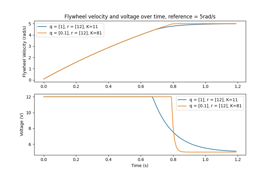
LQR and Measurement Latency Compensation
Oftentimes, our sensors have a delay associated with their measurements. For example the SPARK MAX motor controller over CAN can have up to 30ms of delay associated with velocity measurements.
This lag means that our feedback controller will be generating voltage commands based on state estimates from the past. This often has the effect of introducing instability and oscillations into our system, as shown in the graph below.
However, we can model our controller to control where the system’s state is delayed into the future. This will reduce the LQR’s gain matrix \(\mathbf{K}\), trading off controller performance for stability. The below formula, which adjusts the gain matrix to account for delay, is also used in frc-characterization.
Multiplying \(\mathbf{K}\) by \(\mathbf{A} - \mathbf{BK}\) essentially advances the gains by one timestep. In this case, we multiply by \(\left(\mathbf{A} - \mathbf{BK}\right)^{\text{delay} / dt}\) to advance the gains by measurement’s delay.
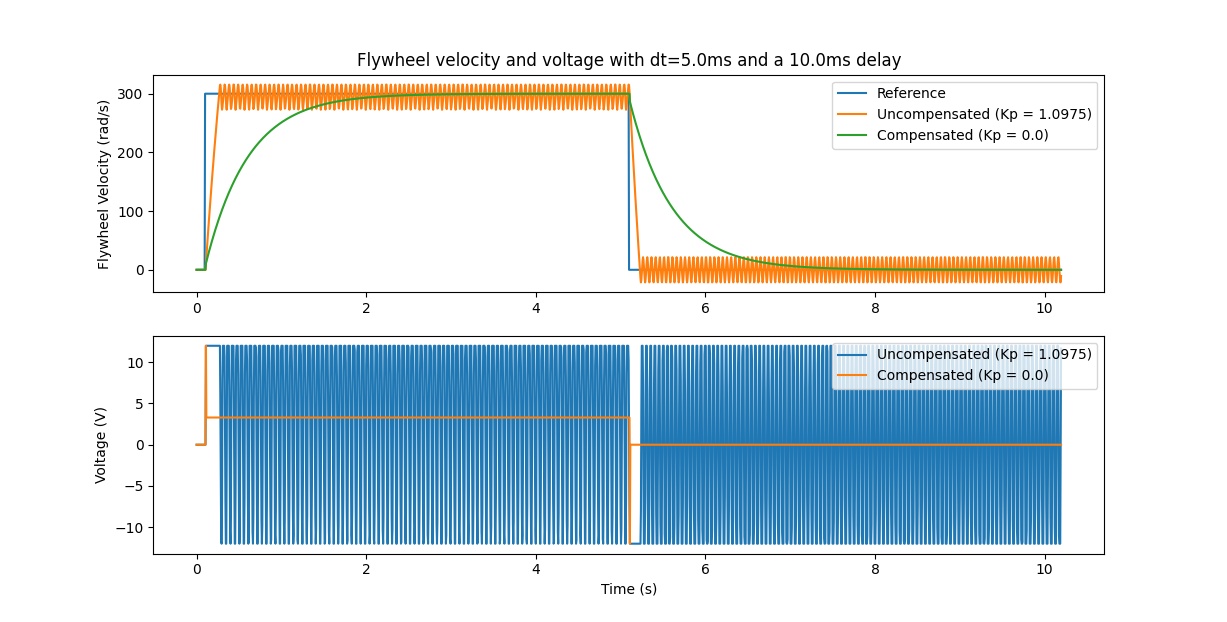
Note
This can have the effect of reducing \(\mathbf{K}\) to zero, effectively disabling feedback control.
Note
The SPARK MAX motor controller uses a 40-tap FIR filter with a delay of 19.5ms, and status frames are by default sent every 20ms.
The code below shows how to adjust the LQR controller’s K gain for sensor input delays:
// Adjust our LQR's controller for 25 ms of sensor input delay. We
// provide the linear system, discretization timestep, and the sensor
// input delay as arguments.
controller.latencyCompensate(elevatorSystem, 0.02, 0.025);
// Adjust our LQR's controller for 25 ms of sensor input delay. We
// provide the linear system, discretization timestep, and the sensor
// input delay as arguments.
controller.LatencyCompensate(elevatorSystem, 20_ms, 25_ms);
Linearization
Linearization is a tool used to approximate nonlinear functions and state-space systems using linear ones. In two-dimensional space, linear functions are straight lines while nonlinear functions curve. A common example of a nonlinear function and its corresponding linear approximation is \(y=\sin{x}\). This function can be approximated by \(y=x\) near zero. This approximation is accurate while near \(x=0\), but looses accuracy as we stray further from the linearization point. For example, the approximation \(\sin{x} \approx x\) is accurate to within 0.02 within 0.5 radians of \(y = 0\), but quickly loses accuracy past that. In the following picture, we see \(y =\sin{x}\), \(y=x\) and the difference between the approximation and the true value of \(\sin{x}\) at \(x\).
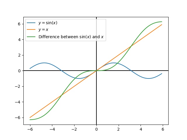
We can also linearize state-space systems with nonlinear dynamics. We do this by picking a point \(\mathbf{x}\) in state-space and using this as the input to our nonlinear functions. Like in the above example, this works well for states near the point about which the system was linearized, but can quickly diverge further from that state.
State-Space Controller Walkthrough
Note
Before following this tutorial, readers are recommended to have read an Introduction to State-Space Control.
The goal of this tutorial is to provide “end-to-end” instructions on implementing a state-space controller for a flywheel. By following this tutorial, readers will learn how to:
Create an accurate state-space model of a flywheel using system identification or CAD software.
Implement a Kalman Filter to filter encoder velocity measurements without lag.
Implement a LQR feedback controller which, when combined with model-based feedforward, will generate voltage inputs to drive the flywheel to a reference.
This tutorial is intended to be approachable for teams without a great deal of programming expertise. While the WPILib library offers significant flexibility in the manner in which its state-space control features are implemented, closely following the implementation outlined in this tutorial should provide teams with a basic structure which can be reused for a variety of state-space systems.
The full example is available in the state-space flywheel (Java/C++) and state-space flywheel system identification (Java/C++) example projects.
Why Use State-Space Control?
Because state-space control focuses on creating an accurate model of our system, we can accurately predict how our model will respond to control inputs. This allows us to simulate our mechanisms without access to a physical robot, as well as easily choose gains that we know will work well. Having a model also allows us to create lagless filters, such as Kalman Filters, to optimally filter sensor readings.
Modeling Our Flywheel
Recall that continuous state-space systems are modeled using the following system of equations:
Where x-dot is the rate of change of the system’s state, \(\mathbf{x}\) is the system’s current state, \(\mathbf{u}\) is the input to the system, and \(\mathbf{y}\) is the sytem’s output.
Let’s use this system of equations to model our flywheel in two different ways. We’ll first model it using system identification using the frc-characterization toolsuite, and then model it based on the motor and flywheel’s moment of inertia.
The first step of building up our state-space system is picking our system’s states. We can pick anything we want as a state – we could pick completely unrelated states if we wanted – but it helps to pick states that are important. We can include hidden states in our state (such as elevator velocity if we were only able to measure its position) and let our Kalman Filter estimate their values. Remember that the states we choose will be driven towards their respective references by the feedback controller (typically the Linear-Quadratic Regulator since it’s optimal).
For our flywheel, we care only about one state: its velocity. While we could chose to also model its acceleration, the inclusion of this state isn’t necessary for our system.
Next, we identify the inputs to our system. Inputs can be thought of as things we can put “into” our system to change its state. In the case of the flywheel (and many other single-jointed mechanisms in FRC®), we have just one input: voltage applied to the motor. By choosing voltage as our input (over something like motor duty cycle), we can compensate for battery voltage sag as battery load increases.
A continuous-time state-space system writes x-dot, or the instantaneous rate of change of the system’s system's state, as proportional to the current state and inputs. Because our state is angular velocity, \(\mathbf{\dot{x}}\) will be the flywheel’s angular acceleration.
Next, we will model our flywheel as a continuous-time state-space system. WPILib’s LinearSystem will convert this to discrete-time internally. Review state-space notation for more on continuous-time and discrete-time systems.
Modeling with System Identification
To rewrite this in state-space notation using system identification, we recall from the flywheel state-space notation example, where we rewrote the following equation in terms of \(\mathbf{a}\).
Where \(\mathbf{v}\) is flywheel velocity, \(\mathbf{a}\) and \(\mathbf{\dot{v}}\) are flywheel acceleration, and \(V\) is voltage. Rewriting this with the standard convention of \(\mathbf{x}\) for the state vector and \(\mathbf{u}\) for the input vector, we find:
The second part of state-space notation relates the system’s current state and inputs to the output. In the case of a flywheel, our output vector \(\mathbf{y}\) (or things that our sensors can measure) is our flywheel’s velocity, which also happens to be an element of our state vector \(\mathbf{x}\). Therefore, our output matrix is \(\mathbf{C} = \begin{bmatrix}1 \end{bmatrix}\), and our system feedthrough matrix is \(\mathbf{D} = \begin{bmatrix}0 \end{bmatrix}\). Writing this out in continuous-time state-space notation yields the following.
The LinearSystem class contains methods for easily creating state-space systems identified using system identification. This example shows a flywheel model with a kV of 0.023 and a kA of 0.001:
33 // Volts per (radian per second)
34 private static final double kFlywheelKv = 0.023;
35
36 // Volts per (radian per second squared)
37 private static final double kFlywheelKa = 0.001;
38
39 // The plant holds a state-space model of our flywheel. This system has the following properties:
40 //
41 // States: [velocity], in radians per second.
42 // Inputs (what we can "put in"): [voltage], in volts.
43 // Outputs (what we can measure): [velocity], in radians per second.
44 //
45 // The Kv and Ka constants are found using the FRC Characterization toolsuite.
46 private final LinearSystem<N1, N1, N1> m_flywheelPlant =
47 LinearSystemId.identifyVelocitySystem(kFlywheelKv, kFlywheelKa);
18
32 // Volts per (radian per second)
33 static constexpr auto kFlywheelKv = 0.023_V / 1_rad_per_s;
34
35 // Volts per (radian per second squared)
36 static constexpr auto kFlywheelKa = 0.001_V / 1_rad_per_s_sq;
37
38 // The plant holds a state-space model of our flywheel. This system has the
39 // following properties:
40 //
41 // States: [velocity], in radians per second.
42 // Inputs (what we can "put in"): [voltage], in volts.
43 // Outputs (what we can measure): [velocity], in radians per second.
44 //
45 // The Kv and Ka constants are found using the FRC Characterization toolsuite.
46 frc::LinearSystem<1, 1, 1> m_flywheelPlant =
47 frc::LinearSystemId::IdentifyVelocitySystem<units::radian>(kFlywheelKv,
48 kFlywheelKa);
Modeling Using Flywheel Moment of Inertia and Gearing
A flywheel can also be modeled without access to a physical robot, using information about the motors, gearing and flywheel’s moment of inertia. A full derivation of this model is presented in Section 8.2.1 of Controls Engineering in FRC.
The LinearSystem class contains methods to easily create a model of a flywheel from the flywheel’s motors, gearing and moment of inertia. The moment of inertia can be calculated using CAD software or using physics. The examples used here are detailed in the flywheel example project (Java/C++).
Note
For WPILib’s state-space classes, gearing is written as output over input – that is, if the flywheel spins slower than the motors, this number should be greater than one.
Note
The C++ LinearSystem class uses the C++ Units Library to prevent unit mixups and assert dimensionality.
34 private static final double kFlywheelMomentOfInertia = 0.00032; // kg * m^2
35
36 // Reduction between motors and encoder, as output over input. If the flywheel spins slower than
37 // the motors, this number should be greater than one.
38 private static final double kFlywheelGearing = 1.0;
39
40 // The plant holds a state-space model of our flywheel. This system has the following properties:
41 //
42 // States: [velocity], in radians per second.
43 // Inputs (what we can "put in"): [voltage], in volts.
44 // Outputs (what we can measure): [velocity], in radians per second.
45 private final LinearSystem<N1, N1, N1> m_flywheelPlant =
46 LinearSystemId.createFlywheelSystem(
47 DCMotor.getNEO(2), kFlywheelMomentOfInertia, kFlywheelGearing);
15#include <frc/system/plant/LinearSystemId.h>
32 static constexpr units::kilogram_square_meter_t kFlywheelMomentOfInertia =
33 0.00032_kg_sq_m;
34
35 // Reduction between motors and encoder, as output over input. If the flywheel
36 // spins slower than the motors, this number should be greater than one.
37 static constexpr double kFlywheelGearing = 1.0;
38
39 // The plant holds a state-space model of our flywheel. This system has the
40 // following properties:
41 //
42 // States: [velocity], in radians per second.
43 // Inputs (what we can "put in"): [voltage], in volts.
44 // Outputs (what we can measure): [velocity], in radians per second.
45 frc::LinearSystem<1, 1, 1> m_flywheelPlant =
46 frc::LinearSystemId::FlywheelSystem(
47 frc::DCMotor::NEO(2), kFlywheelMomentOfInertia, kFlywheelGearing);
Kalman Filters: Observing Flywheel State
Kalman filters are used to filter our velocity measurements using our state-space model to generate a state estimate \(\mathbf{\hat{x}}\). As our flywheel model is linear, we can use a Kalman filter to estimate the flywheel’s velocity. WPILib’s Kalman filter takes a LinearSystem (which we found above), along with standard deviations of model and sensor measurements. We can adjust how “smooth” our state estimate is by adjusting these weights. Larger state standard deviations will cause the filter to “distrust” our state estimate and favor new measurements more highly, while larger measurement standard deviations will do the opposite.
In the case of a flywheel we start with a state standard deviation of 3 rad/s and a measurement standard deviation of 0.01 rad/s. These values are up to the user to choose – these weights produced a filter that was tolerant to some noise but whose state estimate quickly reacted to external disturbances for a flywheel – and should be tuned to create a filter that behaves well for your specific flywheel. Graphing states, measurements, inputs, references, and outputs over time is a great visual way to tune Kalman filters.
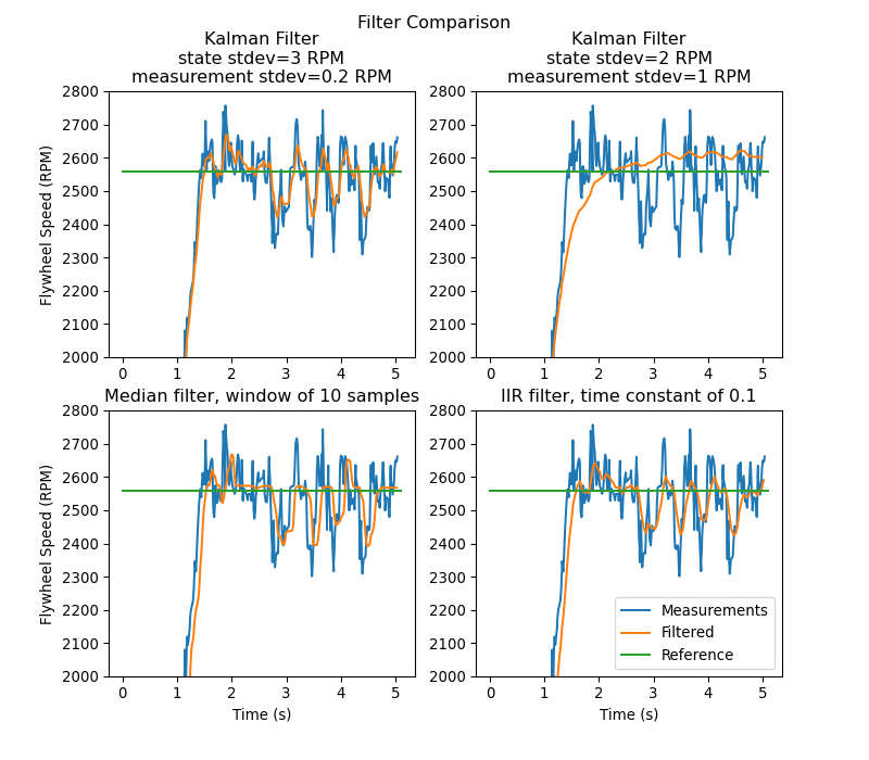
The above graph shows two differently tuned Kalman filters, as well as a single-pole IIR filter and a Median Filter. This data was collected with a shooter over ~5 seconds, and four balls were run through the shooter (as seen in the four dips in velocity). While there are no hard rules on choosing good state and measurement standard deviations, they should in general be tuned to trust the model enough to reject noise while reacting quickly to external disturbances.
Because the feedback controller computes error using the x-hat estimated by the Kalman filter, the controller will react to disturbances only as quickly the filter’s state estimate changes. In the above chart, the upper left plot (with a state standard deviation of 3.0 and measurement standard deviation of 0.2) produced a filter that reacted quickly to disturbances while rejecting noise, while the upper right plot shows a filter that was barely affected by the velocity dips.
59 // The observer fuses our encoder data and voltage inputs to reject noise.
60 private final KalmanFilter<N1, N1, N1> m_observer =
61 new KalmanFilter<>(
62 Nat.N1(),
63 Nat.N1(),
64 m_flywheelPlant,
65 VecBuilder.fill(3.0), // How accurate we think our model is
66 VecBuilder.fill(0.01), // How accurate we think our encoder
67 // data is
68 0.020);
12#include <frc/estimator/KalmanFilter.h>
47 // The observer fuses our encoder data and voltage inputs to reject noise.
48 frc::KalmanFilter<1, 1, 1> m_observer{
49 m_flywheelPlant,
50 {3.0}, // How accurate we think our model is
51 {0.01}, // How accurate we think our encoder data is
52 20_ms};
Because Kalman filters use our state-space model in the Predict step, it is important that our model is as accurate as possible. One way to verify this is to record a flywheel’s input voltage and velocity over time, and replay this data by calling only predict on the Kalman filter. Then, the kV and kA gains (or moment of inertia and other constants) can be adjusted until the model closely matches the recorded data.
Linear-Quadratic Regulators and Plant Inversion Feedforward
The Linear-Quadratic Regulator finds a feedback controller to drive our flywheel system to its reference. Because our flywheel has just one state, the control law picked by our LQR will be in the form \(\mathbf{u = K (r - x)}\) where \(\mathbf{K}\) is a 1x1 matrix; in other words, the control law picked by LQR is simply a proportional controller, or a PID controller with only a P gain. This gain is chosen by our LQR based on the state excursion and control efforts we pass it. More on tuning LQR controllers can be found in the LQR application example.
Much like SimpleMotorFeedforward can be used to generate feedforward voltage inputs given kS, kV, and kA constants, the Plant Inversion Feedforward class generate feedforward voltage inputs given a state-space system. The voltage commands generated by the LinearSystemLoop class are the sum of the feedforward and feedback inputs.
60 // A LQR uses feedback to create voltage commands.
61 private final LinearQuadraticRegulator<N1, N1, N1> m_controller =
62 new LinearQuadraticRegulator<>(
63 m_flywheelPlant,
64 VecBuilder.fill(8.0), // qelms. Velocity error tolerance, in radians per second. Decrease
65 // this to more heavily penalize state excursion, or make the controller behave more
66 // aggressively.
67 VecBuilder.fill(12.0), // relms. Control effort (voltage) tolerance. Decrease this to more
68 // heavily penalize control effort, or make the controller less aggressive. 12 is a good
69 // starting point because that is the (approximate) maximum voltage of a battery.
70 0.020); // Nominal time between loops. 0.020 for TimedRobot, but can be
71 // lower if using notifiers.
10#include <frc/controller/LinearPlantInversionFeedforward.h>
11#include <frc/controller/LinearQuadraticRegulator.h>
54 // A LQR uses feedback to create voltage commands.
55 frc::LinearQuadraticRegulator<1, 1> m_controller{
56 m_flywheelPlant,
57 // qelms. Velocity error tolerance, in radians per second. Decrease this
58 // to more heavily penalize state excursion, or make the controller behave
59 // more aggressively.
60 {8.0},
61 // relms. Control effort (voltage) tolerance. Decrease this to more
62 // heavily penalize control effort, or make the controller less
63 // aggressive. 12 is a good starting point because that is the
64 // (approximate) maximum voltage of a battery.
65 {12.0},
66 // Nominal time between loops. 20ms for TimedRobot, but can be lower if
67 // using notifiers.
68 20_ms};
69
70 // The state-space loop combines a controller, observer, feedforward and plant
71 // for easy control.
72 frc::LinearSystemLoop<1, 1, 1> m_loop{m_flywheelPlant, m_controller,
73 m_observer, 12_V, 20_ms};
Bringing it All Together: LinearSystemLoop
LinearSystemLoop combines our system, controller, and observer that we created earlier. The constructor shown will also instantiate a PlantInversionFeedforward.
73 // The state-space loop combines a controller, observer, feedforward and plant for easy control.
74 private final LinearSystemLoop<N1, N1, N1> m_loop =
75 new LinearSystemLoop<>(m_flywheelPlant, m_controller, m_observer, 12.0, 0.020);
14#include <frc/system/LinearSystemLoop.h>
70 // The state-space loop combines a controller, observer, feedforward and plant
71 // for easy control.
72 frc::LinearSystemLoop<1, 1, 1> m_loop{m_flywheelPlant, m_controller,
73 m_observer, 12_V, 20_ms};
Once we have our LinearSystemLoop, the only thing left to do is actually run it. To do that, we’ll periodically update our Kalman filter with our new encoder velocity measurements and apply new voltage commands to it. To do that, we first set the reference, then correct with the current flywheel speed, predict the Kalman filter into the next timestep, and apply the inputs generated using getU.
96 @Override
97 public void teleopPeriodic() {
98 // Sets the target speed of our flywheel. This is similar to setting the setpoint of a
99 // PID controller.
100 if (m_joystick.getTriggerPressed()) {
101 // We just pressed the trigger, so let's set our next reference
102 m_loop.setNextR(VecBuilder.fill(kSpinupRadPerSec));
103 } else if (m_joystick.getTriggerReleased()) {
104 // We just released the trigger, so let's spin down
105 m_loop.setNextR(VecBuilder.fill(0.0));
106 }
107
108 // Correct our Kalman filter's state vector estimate with encoder data.
109 m_loop.correct(VecBuilder.fill(m_encoder.getRate()));
110
111 // Update our LQR to generate new voltage commands and use the voltages to predict the next
112 // state with out Kalman filter.
113 m_loop.predict(0.020);
114
115 // Send the new calculated voltage to the motors.
116 // voltage = duty cycle * battery voltage, so
117 // duty cycle = voltage / battery voltage
118 double nextVoltage = m_loop.getU(0);
119 m_motor.setVoltage(nextVoltage);
120 }
121}
5#include <frc/DriverStation.h>
6#include <frc/Encoder.h>
7#include <frc/TimedRobot.h>
8#include <frc/XboxController.h>
9#include <frc/controller/LinearPlantInversionFeedforward.h>
10#include <frc/controller/LinearQuadraticRegulator.h>
11#include <frc/drive/DifferentialDrive.h>
12#include <frc/estimator/KalmanFilter.h>
13#include <frc/motorcontrol/PWMSparkMax.h>
14#include <frc/system/LinearSystemLoop.h>
15#include <frc/system/plant/DCMotor.h>
16#include <frc/system/plant/LinearSystemId.h>
17#include <wpi/numbers>
91 void TeleopPeriodic() override {
92 // Sets the target speed of our flywheel. This is similar to setting the
93 // setpoint of a PID controller.
94 if (m_joystick.GetRightBumper()) {
95 // We pressed the bumper, so let's set our next reference
96 m_loop.SetNextR(Eigen::Vector<double, 1>{kSpinup.value()});
97 } else {
98 // We released the bumper, so let's spin down
99 m_loop.SetNextR(Eigen::Vector<double, 1>{0.0});
100 }
101
102 // Correct our Kalman filter's state vector estimate with encoder data.
103 m_loop.Correct(Eigen::Vector<double, 1>{m_encoder.GetRate()});
104
105 // Update our LQR to generate new voltage commands and use the voltages to
106 // predict the next state with out Kalman filter.
107 m_loop.Predict(20_ms);
108
109 // Send the new calculated voltage to the motors.
110 // voltage = duty cycle * battery voltage, so
111 // duty cycle = voltage / battery voltage
112 m_motor.SetVoltage(units::volt_t(m_loop.U(0)));
113 }
State Observers and Kalman Filters
State observers combine information about a system’s behavior and external measurements to estimate the true state of the system. A common observer used for linear systems is the Kalman Filter. Kalman filters are advantageous over other filters as they fuse measurements from one or more sensors with a state-space model of the system to optimally estimate a system’s state.
This image shows flywheel velocity measurements over time, run through a variety of different filters. Note that a well-tuned Kalman filter shows no measurement lag during flywheel spinup while still rejecting noisy data and reacting quickly to disturbances as balls pass through it. More on filters can be found in the filters section.
Gaussian Functions
Kalman filters utilize Gaussian distributions (or bell curves) to model the noise in a process. The graph of a Gaussian function is a “bell curve” shape. This function is described by its mean (the location of the “peak” of the bell curve) and variance (a measure of how “spread out” the bell curve is). In the case of a Kalman filter, the estimated state of the system is the mean, while the variance is a measure of how certain (or uncertain) the filter is about the true state.
The idea of variance and covariance is central to the function of a Kalman filter. Covariance is a measurement of how two random variables are correlated. In a system with a single state, the covariance matrix is simply \(\mathbf{\text{cov}(x_1, x_1)}\), or a matrix containing the variance \(\mathbf{\text{var}(x_1)}\) of the state \(x_1\). The magnitude of this variance is the square of the standard deviation of the Gaussian function describing the current state estimate. Relatively large values for covariance might indicate noisy data, while small covariances might indicate that the filter is more confident about it’s estimate. Remember that “large” and “small” values for variance or covariance are relative to the base unit being used – for example, if \(\mathbf{x_1}\) was measured in meters, \(\mathbf{\text{cov}(x_1, x_1)}\) would be in meters squared.
Covariance matrices are written in the following form:
Kalman Filters
Important
It is important to develop an intuition for what a Kalman filter is actually doing. The book Kalman and Bayesian Filters in Python by Roger Labbe provides a great visual and interactive introduction to Bayesian filters. The Kalman filters in WPILib use linear algebra to gentrify the math, but the ideas are similar to the single-dimensional case. We suggest reading through Chapter 4 to gain an intuition for what these filters are doing.
To summarize, Kalman filters (and all Bayesian filters) have two parts: prediction and correction. Prediction projects our state estimate forward in time according to our system’s dynamics, and correct steers the estimated state towards the measured state. While filters often preform both in the same timestep, it’s not strictly necessary – For example, WPILib’s pose estimators call predict frequently, and correct only when new measurement data is available (for example, from a low-framerate vision system).
The following shows the equations of a discrete-time Kalman filter:
The state estimate \(\mathbf{x}\), together with \(\mathbf{P}\), describe the mean and covariance of the Gaussian function that describes our filter’s estimate of the system’s true state.
Process and Measurement Noise Covariance Matrices
The process and measurement noise covariance matrices \(\mathbf{Q}\) and \(\mathbf{R}\) describe the variance of each of our states and measurements. Remember that for a Gaussian function, variance is the square of the function’s standard deviation. In a WPILib, Q and R are diagonal matrices whose diagonals contain their respective variances. For example, a Kalman filter with states \(\begin{bmatrix}\text{position} \\ \text{velocity} \end{bmatrix}\) and measurements \(\begin{bmatrix}\text{position} \end{bmatrix}\) with state standard deviations \(\begin{bmatrix}0.1 \\ 1.0\end{bmatrix}\) and measurement standard deviation \(\begin{bmatrix}0.01\end{bmatrix}\) would have the following \(\mathbf{Q}\) and \(\mathbf{R}\) matrices:
Error Covariance Matrix
The error covariance matrix \(\mathbf{P}\) describes the covariance of the state estimate \(\mathbf{\hat{x}}\). Informally, \(\mathbf{P}\) describes our certainty about the estimated state. If \(\mathbf{P}\) is large, our uncertainty about the true state is large. Conversely, a \(\mathbf{P}\) with smaller elements would imply less uncertainty about our true state.
As we project the model forward, \(\mathbf{P}\) increases as our certainty about the system’s true state decreases.
Predict step
In prediction, our state estimate is updated according to the linear system dynamics \(\mathbf{\dot{x} = Ax + Bu}\). Furthermore, our error covariance \(\mathbf{P}\) increases by the process noise covariance matrix \(\mathbf{Q}\). Larger values of \(\mathbf{Q}\) will make our error covariance \(\mathbf{P}\) grow more quickly. This \(\mathbf{P}\) is used in the correction step to weight the model and measurements.
Correct step
In the correct step, our state estimate is updated to include new measurement information. This new information is weighted against the state estimate \(\mathbf{\hat{x}}\) by the Kalman gain \(\mathbf{K}\). Large values of \(\mathbf{K}\) more highly weight incoming measurements, while smaller values of \(\mathbf{K}\) more highly weight our state prediction. Because \(\mathbf{K}\) is related to \(\mathbf{P}\), larger values of \(\mathbf{P}\) will increase \(\mathbf{K}\) and more heavily weight measurements. If, for example, a filter is predicted for a long duration, the large \(\mathbf{P}\) would heavily weight the new information.
Finally, the error covariance \(\mathbf{P}\) decreases to increase our confidence in the state estimate.
Tuning Kalman Filters
WPILib’s Kalman Filter classes’ constructors take a linear system, a vector of process noise standard deviations and measurement noise standard deviations. These are converted to \(\mathbf{Q}\) and \(\mathbf{R}\) matrices by filling the diagonals with the square of the standard deviations, or variances, of each state or measurement. By decreasing a state’s standard deviation (and therefore its corresponding entry in \(\mathbf{Q}\)), the filter will distrust incoming measurements more. Similarly, increasing a state’s standard deviation will trust incoming measurements more. The same holds for the measurement standard deviations – decreasing an entry will make the filter more highly trust the incoming measurement for the corresponding state, while increasing it will decrease trust in the measurement.
49 // The observer fuses our encoder data and voltage inputs to reject noise.
50 private final KalmanFilter<N1, N1, N1> m_observer =
51 new KalmanFilter<>(
52 Nat.N1(),
53 Nat.N1(),
54 m_flywheelPlant,
55 VecBuilder.fill(3.0), // How accurate we think our model is
56 VecBuilder.fill(0.01), // How accurate we think our encoder
57 // data is
58 0.020);
5#include <frc/DriverStation.h>
6#include <frc/Encoder.h>
7#include <frc/TimedRobot.h>
8#include <frc/XboxController.h>
9#include <frc/controller/LinearQuadraticRegulator.h>
10#include <frc/drive/DifferentialDrive.h>
11#include <frc/estimator/KalmanFilter.h>
12#include <frc/motorcontrol/PWMSparkMax.h>
13#include <frc/system/LinearSystemLoop.h>
14#include <frc/system/plant/DCMotor.h>
15#include <frc/system/plant/LinearSystemId.h>
16#include <units/angular_velocity.h>
17#include <wpi/numbers>
47 // The observer fuses our encoder data and voltage inputs to reject noise.
48 frc::KalmanFilter<1, 1, 1> m_observer{
49 m_flywheelPlant,
50 {3.0}, // How accurate we think our model is
51 {0.01}, // How accurate we think our encoder data is
52 20_ms};
WPILib Pose Estimators
WPILib includes pose estimators for differential, swerve and mecanum drivetrains. These estimators are designed to be drop-in replacements for the existing odometry classes, with added features that utilize an Unscented Kalman Filter to fuse latency-compensated robot pose estimates with encoder and gyro measurements. These estimators can account for encoder drift and noisy vision data. These estimators can behave identically to their corresponding odometry classes if only update is called on these estimators.
Pose estimators estimate robot position using a state-space system with the states \(\begin{bmatrix}x & y & \theta \end{bmatrix}^T\), which can represent robot position as a Pose2d. WPILib includes DifferentialDrivePoseEstimator, SwerveDrivePoseEstimator and MecanumDrivePoseEstimator to estimate robot position. In these, users call update periodically with encoder and gyro measurements (same as the odometry classes) to update the robot’s estimated position. When the robot receives measurements of its field-relative position (encoded as a Pose2d) from sensors such as computer vision or V-SLAM, the pose estimator latency-compensates the measurement to accurately estimate robot position.
The pose estimators perform latency compensation by storing a list of past observer states, including estimated state \(\mathbf{\hat{x}}\), error covariance \(\mathbf{P}\), inputs and local measurements. When new measurements are applied, the state of the estimator is first rolled back to the measurement’s timestamp. Then, the filter corrects its state estimate with the new measurement and applies the inputs between the measurement timestamp and the present time to incorporate the new measurement. This allows for vision solutions with framerates which might otherwise make them unusable be a viable solution for robot localization.
The following example shows the use of the DifferentialDrivePoseEstimator:
var estimator = new DifferentialDrivePoseEstimator(new Rotation2d(), new Pose2d(),
new MatBuilder<>(Nat.N5(), Nat.N1()).fill(0.02, 0.02, 0.01, 0.02, 0.02), // State measurement standard deviations. X, Y, theta.
new MatBuilder<>(Nat.N3(), Nat.N1()).fill(0.02, 0.02, 0.01), // Local measurement standard deviations. Left encoder, right encoder, gyro.
new MatBuilder<>(Nat.N3(), Nat.N1()).fill(0.1, 0.1, 0.01)); // Global measurement standard deviations. X, Y, and theta.
#include "frc/estimator/DifferentialDrivePoseEstimator.h"
#include "frc/StateSpaceUtil.h"
frc::DifferentialDrivePoseEstimator estimator{
frc::Rotation2d(), frc::Pose2d(),
frc::MakeMatrix<5, 1>(0.01, 0.01, 0.01, 0.01, 0.01),
frc::MakeMatrix<3, 1>(0.1, 0.1, 0.1),
frc::MakeMatrix<3, 1>(0.1, 0.1, 0.1)};
Tuning Pose Estimators
All pose estimators offer user-customizable standard deviations for model and measurements. These standard deviations determine how much the filter “trusts” each of these states. For example, increasing the standard deviation for measurements (as one might do for a noisy signal) would lead to the estimator trusting its state estimate more than the incoming measurements. On the field, this might mean that the filter can reject noisy vision data well, at the cost of being slow to correct for model deviations. While these values can be estimated beforehand, they very much depend on the unique setup of each robot and global measurement method.
Debugging State-Space Models and Controllers
Checking Signs
One of the most common causes of bugs with state-space controllers is signs being flipped. For example, models included in WPILib expect positive voltage to result in a positive acceleration, and vice versa. If applying a positive voltage does not make the mechanism accelerate forwards, or if moving “forwards” makes encoder (or other sensor readings) decrease, they should be inverted so that positive voltage input results in a positive encoder reading. For example, if I apply an input of \([12, 12]^T\) (full forwards for the left and right motors) to my differential drivetrain, my wheels should propel my robot “forwards” (along the +X axis locally), and for my encoders to read a positive velocity.
Important
The WPILib DifferentialDrive by default inverts the right motors. This behavior can be changed by calling setRightSideInverted(false)/SetRightSideInverted(false) (Java/C++) on the DifferentialDrive object.
The Importance of Graphs
Reliable data of the system’s states, inputs and outputs over time is important when debugging state-space controllers and observers. One common approach is to send this data over NetworkTables and use tools such as Shuffleboard, which allow us to both graph the data in real-time as well as save it to a CSV file for plotting later with tools such as Google Sheets, Excel or Python.
Note
By default, NetworkTables is limited to a 10hz update rate. For testing, this can be bypassed with the following code snippet to submit data at up to 100hz. This code should be run periodically to forcibly publish new data.
Danger
This will send extra data (at up to 100hz) over NetworkTables, which can cause lag with both user code and robot dashboards. This will also increase network utilization. It is often a good idea to disable this during competitions.
@Override
public void robotPeriodic() {
NetworkTableInstance.getDefault().flush();
}
void RobotPeriodic() {
NetworkTableInstance::GetDefault().Flush();
}
Compensating for Input Lag
Often times, some sensor input data (i.e. velocity readings) may be delayed due to onboard filtering that smart motor controllers tend to perform. By default, LQR’s K gain assumes no input delay, so introducing significant delay on the order of tens of milliseconds can cause instability. To combat this, the LQR’s K gain can be reduced, trading off performance for stability. A code example for how to compensate for this latency in a mathematically rigorous manner is available here.
Controls Glossary
- control effort
A term describing how much force, pressure, etc. an actuator is exerting.
- control input
The input of a plant used for the purpose of controlling it
- control law
A mathematical formula that generates inputs to drive a system to a desired state, given the current state. A common example is the control law \(\mathbf{u} = \mathbf{K(r - x)}\)
- controller
Used in position or negative feedback with a plant to bring about a desired system state by driving the difference between a reference signal and the output to zero.
- dynamics
A branch of physics concerned with the motion of bodies under the action of forces. In modern control, systems evolve according to their dynamics.
- error
- gain
A proportional value that relates the magnitude of an input signal to the magnitude of an output signal. In the signal-dimensional case, gain can be thought of as the proportional term of a PID controller. A gain greater than one would amplify an input signal, while a gain less than one would dampen an input signal. A negative gain would negate the input signal.
A state that cannot be directly measured, but whose dynamics can be related to other states.
- input
An input to the plant (hence the name) that can be used to change the plant’s state.
Ex. A flywheel will have 1 input: the voltage of the motor driving it.
Ex. A drivetrain might have 2 inputs: the voltages of the left and right motors.
Inputs are often represented by the variable \(\mathbf{u}\), a column vector with one entry per input to the system.
- measurement
Measurements are outputs that are measured from a plant, or physical system, using sensors.
- model
A set of mathematical equations that reflects some aspect of a physical system’s behavior.
- moment of inertia
A measurement of a rotating body’s resistance to angular acceleration or deceleration. Angular moment of inertia can be thought of as angular mass. See also: Moment of inertia.
- observer
In control theory, a system that provides an estimate of the internal state of a given real system from measurements of the input and output of the real system. WPILib includes a Kalman Filter class for observing linear systems, and ExtendedKalmanFilter and UnscentedKalmanFilter classes for nonlinear systems.
- output
Measurements from sensors. There can be more measurements then states. These outputs are used in the “correct” step of Kalman Filters.
Ex. A flywheel might have 1 output from a encoder that measures it’s velocity.
Ex. A drivetrain might use solvePNP and V-SLAM to find it’s x/y/heading position on the field. It’s fine that there are 6 measurements (solvePNP x/y/heading and V-SLAM x/y/heading) and 3 states (robot x/y/heading).
Outputs of a system are often represented using the variable \(\mathbf{y}\), a column vector with one entry per output (or thing we can measure). For example, if our system had states for velocity and acceleration but our sensor could only measure velocity, our, our output vector would only include the system's velocity.
- plant
The system or collection of actuators being controlled.
- process variable
The term used to describe the output of a plant in the context of PID control.
- reference
The desired state. This value is used as the reference point for a controller’s error calculation.
- rise time
The time a system takes to initially reach the reference after applying a step input.
- setpoint
The term used to describe the reference of a PID controller.
- settling time
The time a system takes to settle at the reference after a step input is applied.
- state
A characteristic of a system (e.g., velocity) that can be used to determine the system’s future behavior. In state-space notation, the state of a system is written as a column vector describing it’s position in state-space.
Ex. A drivetrain system might have the states \(\begin{bmatrix}x \\ y \\ \theta \end{bmatrix}\) to describe it’s position on the field.
Ex. An elevator system might have the states \(\begin{bmatrix} \text{position} \\ \text{velocity} \end{bmatrix}\) to describe its current height and velocity.
A system’s state is often represented by the variable \(\mathbf{x}\), a column vector with one entry per state.
- steady-state error
- step input
A system input that is \(0\) for \(t < 0\) and a constant greater than \(0\) for \(t \geq 0\). A step input that is \(1\) for \(t \geq 0\) is called a unit step input.
- step response
The response of a system to a step input.
- system
A term encompassing a plant and it’s interaction with a controller and observer, which is treated as a single entity. Mathematically speaking, a system maps inputs to outputs through a linear combination of states.
- system identification
The process of capturing a systems dynamics in a mathematical model using measured data. The characterization toolsuite uses system identification to find kS, kV and kA terms.
- system response
- x-dot
\(\dot{\mathbf{x}}\), or x-dot: the derivative of the state vector \(\mathbf{x}\). If the system had just a velocity state, then \(\dot{\mathbf{x}}\) would represent the system's acceleration.
- x-hat
\(\hat{\mathbf{x}}\), or x-hat: the estimated state of a system, as estimated by an observer.
Convenience Features
This section covers some general convenience features that be used with other advanced programming features.
Scheduling Functions at Custom Frequencies
TimedRobot’s addPeriodic() method allows one to run custom methods at a rate faster than the default TimedRobot periodic update rate (20 ms). Previously, teams had to make a Notifier to run feedback controllers more often than the TimedRobot loop period of 20 ms (running TimedRobot more often than this is not advised). Now, users can run feedback controllers more often than the main robot loop, but synchronously with the TimedRobot periodic functions, eliminating potential thread safety issues.
The addPeriodic() (Java) / AddPeriodic() (C++) method takes in a lambda (the function to run), along with the requested period and an optional offset from the common starting time. The optional third argument is useful for scheduling a function in a different timeslot relative to the other TimedRobot periodic methods.
Note
The units for the period and offset are seconds in Java. In C++, the units library can be used to specify a period and offset in any time unit.
public class Robot extends TimedRobot {
private Joystick m_joystick = new Joystick(0);
private Encoder m_encoder = new Encoder(1, 2);
private Spark m_motor = new Spark(1);
private PIDController m_controller = new PIDController(1.0, 0.0, 0.5, 0.01);
public Robot() {
addPeriodic(() -> {
m_motor.set(m_controller.calculate(m_encoder.getRate()));
}, 0.01, 0.005);
}
@Override
public teleopPeriodic() {
if (m_joystick.getRawButtonPressed(1)) {
if (m_controller.getSetpoint() == 0.0) {
m_controller.setSetpoint(30.0);
} else {
m_controller.setSetpoint(0.0);
}
}
}
}
class Robot : public frc::TimedRobot {
private:
frc::Joystick m_joystick{0};
frc::Encoder m_encoder{1, 2};
frc::Spark m_motor{1};
frc2::PIDController m_controller{1.0, 0.0, 0.5, 10_ms};
Robot();
void TeleopPeriodic() override;
};
void Robot::Robot() {
AddPeriodic([&] {
m_motor.Set(m_controller.Calculate(m_encoder.GetRate()));
}, 10_ms, 5_ms);
}
void Robot::TeleopPeriodic() {
if (m_joystick.GetRawButtonPressed(1)) {
if (m_controller.GetSetpoint() == 0.0) {
m_controller.SetSetpoint(30.0);
} else {
m_controller.SetSetpoint(0.0);
}
}
}
The teleopPeriodic() method in this example runs every 20 ms, and the controller update is run every 10 ms with an offset of 5 ms from when teleopPeriodic() runs so that their timeslots don’t conflict (e.g., teleopPeriodic() runs at 0 ms, 20 ms, 40 ms, etc.; the controller runs at 5 ms, 15 ms, 25 ms, etc.).
WPILib Example Projects
Warning
While every attempt is made to keep WPILib examples functional, they are not intended to be used “as-is.” At the very least, robot-specific constants will need to be changed for the code to work on a user robot. Many empirical constants have their values “faked” for demonstration purposes. Users are strongly encouraged to write their own code (from scratch or from an existing template) rather than copy example code.
WPILib example projects demonstrate a large number of library features and use patterns. Projects range from simple demonstrations of a single functionality to complete, competition-capable robot programs. All of these examples are available in VS Code by entering Ctrl+Shift+P, then selecting WPILib: Create a new project and choosing example.
Basic Examples
These examples demonstrate basic/minimal robot functionality. They are useful for beginning teams who are gaining initial familiarity with robot programming, but are highly limited in functionality.
Arcade Drive (Java, C++): Demonstrates a simple differential drive implementation using “arcade”-style controls through the
DifferentialDriveclass.Arcade Drive Xbox Controller (Java, C++): Demonstrates the same functionality seen in the previous example, except using an
XboxControllerinstead of an ordinary joystick.Getting Started (Java, C++): Demonstrates a simple autonomous routine that drives forwards for two seconds at half speed.
Mecanum Drive (Java, C++): Demonstrates a simple mecanum drive implementation using the
MecanumDriveclass.Motor Controller (Java, C++): Demonstrates how to control the output of a motor with a joystick.
Motor Control With Encoder (Java, C++): Identical to the above example, except with the addition of an encoder to read the motor position.
Simple Vision (Java, C++): Demonstrates how to stream video from a USB camera to the dashboard.
Relay (Java, C++): Demonstrates the use of the
Relayclass to control a relay output with a set of joystick buttons.Solenoids (Java, C++): Demonstrates the use of the
SolenoidandDoubleSolenoidclasses to control solenoid outputs with a set of joystick buttons.TankDrive (Java, C++): Demonstrates a simple differential drive implementation using “tank”-style controls through the
DifferentialDriveclass.Tank Drive Xbox Controller (Java, C++): Demonstrates the same functionality seen in the previous example, except using an
XboxControllerinstead of an ordinary joystick.
Control Examples
These examples demonstrate WPILib implementations of common robot controls. Sensors may be present, but are not the emphasized concept of these examples.
DifferentialDriveBot (Java, C++): Demonstrates an advanced differential drive implementation, including encoder-and-gyro odometry through the
DifferentialDriveOdometryclass, and composition with PID velocity control through theDifferentialDriveKinematicsandPIDControllerclasses.Elevator with profiled PID controller (Java, C++): Demonstrates the use of the
ProfiledPIDControllerclass to control the position of an elevator mechanism.Elevator with trapezoid profiled PID (Java, C++): Demonstrates the use of the
TrapezoidProfileclass in conjunction with a “smart motor controller” to control the position of an elevator mechanism.Gyro Mecanum (Java, C++): Demonstrates field-oriented control of a mecanum robot through the
MecanumDriveclass in conjunction with a gyro.MecanumBot (Java, C++): Demonstrates an advanced mecanum drive implementation, including encoder-and-gyro odometry through the
MecanumDriveOdometryclass, and composition with PID velocity control through theMecanumDriveKinematicsandPIDControllerclasses.PotentiometerPID (Java, C++): Demonstrates the use of the
PIDControllerclass and a potentiometer to control the position of an elevator mechanism.RamseteController (Java, C++): Demonstrates the use of the
RamseteControllerclass to follow a trajectory during the autonomous period.SwerveBot (Java, C++): Demonstrates an advanced swerve drive implementation, including encoder-and-gyro odometry through the
SwerveDriveOdometryclass, and composition with PID position and velocity control through theSwerveDriveKinematicsandPIDControllerclasses.UltrasonicPID (Java, C++): Demonstrates the use of the
PIDControllerclass in conjunction with an ultrasonic sensor to drive to a set distance from an object.
Sensor Examples
These examples demonstrate sensor reading and data processing using WPILib. Mechanisms control may be present, but is not the emphasized concept of these examples.
Axis Camera Sample (Java, C++): Demonstrates the use of OpenCV and an Axis Netcam to overlay a rectangle on a captured video feed and stream it to the dashboard.
Power Distribution CAN Monitoring (Java, C++): Demonstrates obtaining sensor information from a Power Distribution module over CAN using the
PowerDistributionclass.Duty Cycle Encoder (Java, C++): Demonstrates the use of the
DutyCycleEncoderclass to read values from a PWM-type absolute encoder.DutyCycleInput (Java, C++): Demonstrates the use of the
DutyCycleInputclass to read the frequency and fractional duty cycle of a PWM input.Encoder (Java, C++): Demonstrates the use of the
Encoderclass to read values from a quadrature encoder.Gyro (Java, C++): Demonstrates the use of the
AnalogGyroclass to measure robot heading and stabilize driving.Intermediate Vision (Java, C++): Demonstrates the use of OpenCV and a USB camera to overlay a rectangle on a captured video feed and stream it to the dashboard.
Ultrasonic (Java, C++): Demonstrates the use of the
Ultrasonicclass to read data from an ultrasonic sensor in conjunction with theMedianFilterclass to reduce signal noise.
Command-Based Examples
These examples demonstrate the use of the Command-Based framework.
ArmBot (Java, C++): Demonstrates the use of a
ProfiledPIDSubsystemto control a robot arm.ArmBotOffboard (Java, C++): Demonstrates the use of a
TrapezoidProfileSubsystemin conjunction with a “smart motor controller” to control a robot arm.DriveDistanceOffboard (Java, C++): Demonstrates the use of a
TrapezoidProfileCommandin conjunction with a “smart motor controller” to drive forward by a set distance with a trapezoidal motion profile.FrisbeeBot (Java, C++): A complete set of robot code for a simple frisbee-shooting robot typical of the 2013 FRC® game Ultimate Ascent. Demonstrates simple PID control through the
PIDSubystemclass.Gears Bot (Java, C++): A complete set of robot code for the WPI demonstration robot, GearsBot.
Gyro Drive Commands (Java, C++): Demonstrates the use of
PIDCommandandProfiledPIDCommandin conjunction with a gyro to turn a robot to face a specified heading and to stabilize heading while driving.Inlined Hatchbot (Java, C++): A complete set of robot code for a simple hatch-delivery bot typical of the 2019 FRC game Destination: Deep Space. Commands are written in an “inline” style, in which explicit subclassing of
Commandis avoided.Traditional Hatchbot (Java, C++): A complete set of robot code for a simple hatch-delivery bot typical of the 2019 FRC game Destination: Deep Space. Commands are written in a “traditional” style, in which subclasses of
Commandare written for each robot action.MecanumControllerCommand (Java, C++): Demonstrates trajectory generation and following with a mecanum drive using the
TrajectoryGeneratorandMecanumControllerCommandclasses.RamseteCommand (Java, C++): Demonstrates trajectory generation and following with a differential drive using the
TrajectoryGeneratorandRamseteCommandclasses. A matching step-by-step tutorial can be found here.Scheduler Event Logging (Java, C++): Demonstrates the use of scheduler event actions to log dashboard event markers whenever a command starts, ends, or is interrupted.
Select Command Example (Java, C++): Demonstrates the use of the
SelectCommandclass to run one of a selection of commands depending on a runtime-evaluated condition.SwerveControllerCommand (Java, C++): Demonstrates trajectory generation and following with a swerve drive using the
TrajectoryGeneratorandSwerveControllerCommandclasses.
State-Space Examples
These examples demonstrate the use of the State-Space Control.
StateSpaceFlywheel (Java, C++): Demonstrates state-space control of a flywheel.
StateSpaceFlywheelSysId (Java, C++): Demonstrates state-space control using FRC Characterization’s System Identification for controlling a flywheel.
StateSpaceElevator (Java, C++): Demonstrates state-space control of an elevator.
StateSpaceArm (Java, C++): Demonstrates state-space control of an Arm.
StateSpaceDriveSimulation (Java, C++): Demonstrates state-space control of a differential drivetrain in combination with a RAMSETE path following controller and Field2d class.
Simulation Physics Examples
These examples demonstrate the use of the physics simulation.
ElevatorSimulation (Java, C++): Demonstrates the use of physics simulation with a simple elevator.
ArmSimulation (Java, C++): Demonstrates the use of physics simulation with a simple single-jointed arm.
StateSpaceDriveSimulation (Java, C++): Demonstrates state-space control of a differential drivetrain in combination with a RAMSETE path following controller and Field2d class.
SimpleDifferentialDriveSimulation (Java, C++): A barebones example of a basic drivetrain that can be used in simulation.
Miscellaneous Examples
These examples demonstrate miscellaneous WPILib functionality that does not fit into any of the above categories.
Addressable LED (Java, C++): Demonstrates the use of the
AddressableLEDclass to control RGB LEDs for robot decoration and/or driver feedback.DMA (C++): Demonstrates the use of DMA (Direct Memory Access) to read from sensors without using the RoboRIO’s CPU (C++ only).
HAL (C++): Demonstrates the use of HAL (Hardware Abstraction Layer) without the use of the rest of WPILib. This example is for advanced users (C++ only).
HID Rumble (Java, C++): Demonstrates the use of the “rumble” functionality for tactile feedback on supported HIDs (such as XboxControllers).
Shuffleboard (Java, C++): Demonstrates configuring tab/widget layouts on the “Shuffleboard” dashboard from robot code through the
Shuffleboardclass’s fluent builder API.RomiReference (Java, C++): A command based example of how to run the Romi robot.
Mechanism2d (Java, C++): A simple example of using Mechanism2d.
Third Party Example Projects
This list helps you find example programs for use with third party devices. You can find support for many of these third parties on the Support Resources page.
Limelight (additional examples, called case studies, can be found on the left)
Hardware - Basics
Wiring Best Practices
Tip
The article Wiring the FRC Control System walks through the details of what connects where to wire up the FRC Control System and this article provides some additional “Best Practices” that may increase reliability and make maintenance easier. Take a look at Preemptive Troubleshooting for more tips and tricks.
Vibration/Shock
An FRC® Robot is an incredibly rough environment when it comes to vibrations and shock loads. While many of the FRC specific electronics are extensively tested for mechanical robustness in these conditions, a few components, such as the radio, are not specifically designed for use on a mobile platform. Taking steps to reduce the shock and vibration these components are exposed to may help reduce failures. Some suggestions that may reduce mechanical failures:
Vibration Isolation - Make sure to isolate any components which create excessive vibration, such as compressors, using “vibration isolators”. This will help reduce vibration on the robot which can loosen fasteners and cause premature fatigue failure on some electronic components.
Bumpers - Use Bumpers to cover as much of the robot as possible for your design. While the rules require specific bumper coverage around the corners of your robot, maximizing the use of bumpers increases the likelihood that all collisions will be damped by your bumpers. Bumpers significantly reduce the g-forces experienced in a collision compared to hitting directly on a hard robot surface, reducing the shock experienced by the electronics and decreasing the chance of a shock related failure.
Shock Mounting - You may choose to shock mount some or all of your electronic components to further reduce the forces they see in robot collisions. This is especially helpful for the robot radio and other electronics such as co-processors, which may not be designed for use on mobile platforms. Vibration isolators, springs, foams, or mounting to flexible materials all may reduce the shock forces seen by these components.
Redundancy
Unfortunately there are few places in the FRC Control System where redundancy is feasible. Taking advantage of opportunities for redundancy can increase reliability. The primary example of this is wiring the barrel connector to the radio in addition to the provided PoE connection. This ensures that if one of the cables becomes damaged or dislodged, the other will maintain power to the radio. Keep an eye out for other potential areas to provide redundancy when wiring and programming your robot.
Port Savers
For any connections on the Robot or Driver station that may be frequently plugged and unplugged (such as DS joysticks, DS Ethernet, roboRIO USB tether, and Ethernet tether) using a “Port Saver” or “pigtail” can substantially reduce the potential for damaging the port. This type of device can serve double duty, both reducing the number of cycles that the port on the electronic device sees, as well as relocating the connection to a more convenient location. Make sure to secure the port saver (see the next item) to avoid port damage.
Wire Management and Strain Relief
One of the most critical components to robot reliability and maintenance is good wire management and strain relief. Good wire management is comprised of a few components:
Make sure cables are the correct length. Any excess wire length is just more to manage. If you must have extra wire due to additional length on COTS cabling, secure the extra into a small bundle using separate cable ties before securing the rest of the wire.
Ensure that cables are secured close to connection points, with enough slack to avoid putting strain on connectors. This is called strain relief, and is critical to minimizing the likelihood that a cable comes unplugged or a wire breaks off at a connection point (these are generally stress concentrators).
Secure cables near any moving components. Make sure that all wire runs are secure and protected from moving components, even if the moving components were to bend or over-travel.
Secure cables at additional points as necessary to keep wiring neat and clean. Take care to not over secure wires; if wires are secured in too many locations, it may actually make troubleshooting and maintenance more difficult.
Documentation
A great way to make maintenance easier is to create documentation describing what is connected where on the robot. There are a number of ways of creating this type of documentation which range from complete wiring diagrams to excel charts to a quick list of what functions are attached to which channels. Many teams also integrate these lists with labeling (see the next bullet).
When a wire is accidentally cut, or a mechanism is malfunctioning, or a component burns out, it will be much easier to repair if you have some documentation to tell you what is connected where without having to trace the wiring all the way through (even if your wiring is neat!)
Labeling
Labeling is a great way to supplement the wiring documentation described above. There are many different strategies to labeling wiring and electronics, all with their own pros and cons. Labels for electronics and flags for wires can be made by hand, or using a label maker (some can also do heat-shrink labels), or you can use different colors of electrical tape or labeling flags to indicate different things. Whatever system you choose, make sure you understand how it complements your documentation and make sure everyone on your team is familiar with it.
Check all wiring and connections
After all wiring on the robot is complete, make sure to check each connection, pulling on each, to ensure that everything is secure. Additionally, ensure that no stray wire “whiskers” are sticking out of any connection point and that no uninsulated connections are exposed. If any connections come loose while testing, or any “whiskers” are discovered, re-make the connection and make sure to have a second person check it when complete.
A common source of poor connections is screw-type or nut-and-bolt fasteners. For any connections of this type on the robot (e.g. battery connections, main breaker, PDP, roboRIO), make sure the fasteners are tight. For nut-and-bolt style connections, ensure that the wire/terminal cannot be rotate by hand; if you can rotate your battery wire or main breaker connection by grasping the terminal and twisting, the connection is not tight enough.
Another common source of failures is the fuses at the end of the PDP. Ensure these fuses are completely seated; you may need to apply more force than you expect to seat them completely. If the fuses are seated properly they will likely be difficult or impossible to remove by hand.
Snap-in connections such as the SB-50 connector should be secured using clips or cable ties to ensure they do not pop loose during impacts.
Re-Check Early and Often
Re-check the entire electrical system as thoroughly as possible after playing the first match or two (or doing very vigorous testing). The first few impacts the robot sees may loosen fasteners or expose issues.
Create a checklist for re-checking electrical connections on a regular basis. As a very rough starting point, rotational fasteners such as battery and PDP connections should be checked every 1-3 matches. Spring type connections such as the WAGO and Weidmuller connectors likely only need to be checked once per event. Ensure that the team knows who is responsible for completing the checklist and how they will document that it has been done.
Battery Maintenance
Take good care of your batteries! A bad battery can easily cause a robot to functional poorly, or not at all, during a match. Label all of your batteries to help keep track of usage during the event. Many teams also include information such as the age of the battery on this label.
Never lift or carry batteries by the wires! Carrying batteries by the wires has the potential to damage the internal connection between the terminals and the plates, dramatically increasing internal resistance and degrading performance.
Mark any dropped battery bad until a complete test can be conducted. In addition to the mentioned terminal connections, dropping a battery also has the potential to damage individual cells. This damage may not register on a simple voltage test, instead hiding until the battery is placed under load.
Rotate batteries evenly. This helps ensure that batteries have the most time to charge and rest and that they wear evenly (equal number of charge/discharge cycles)
Load test batteries if possible to monitor health. There are a number of commercially available products teams use to load test batteries, including at least one designed specifically for FRC. A load test can provide an indicator of battery health by measuring internal resistance. This measurement is much more meaningful when it comes to match performance than a simple no-load voltage number provided by a multimeter.
Check DS Logs
After each match, review the DS logs to see what the battery voltage and current usage looks like. Once you have established what the normal range of these items is for your robot, you may be able to spot potential issues (bad batteries, failing motors, mechanical binding) before they become critical failures.
CAN Wiring Basics
CAN is a two wire network that is designed to facilitate communication between multiple devices on your robot. It is recommended that CAN on your robot follow a “daisy-chain” topology. This means that the CAN wiring should usually start at your roboRIO and go into and out of each device successively until finally ending at the PDP.
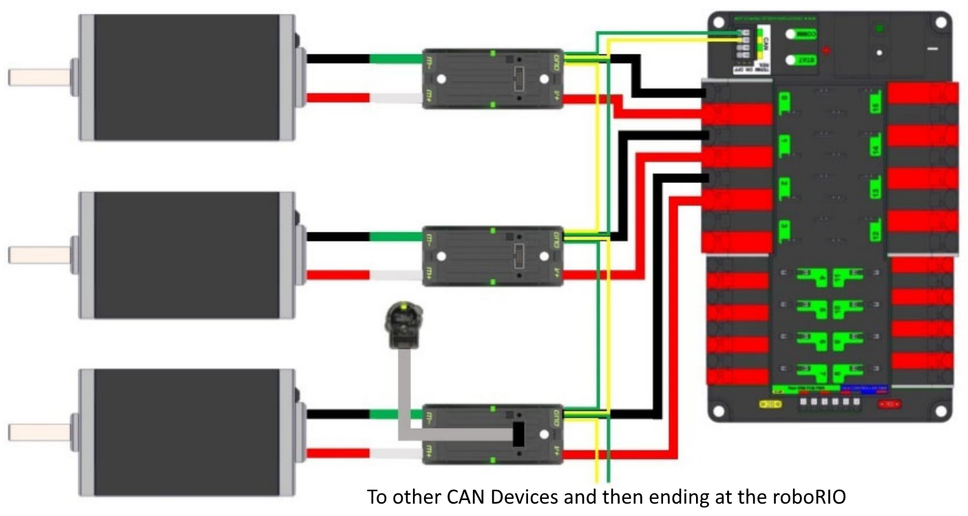
Standard Wiring
CAN is generally wired with yellow and green wire with yellow acting as the CAN-High and green as the CAN-Low signals. Many devices show this yellow and green color scheme to indicate how the wires should be plugged in.
CAN wiring from the roboRIO to the PCM.
CAN wiring from the PCM to the PDP.
Termination
It is recommended that the wiring starts at the roboRIO and ends at the PDP because the CAN network is required to be terminated by 120 \(\Omega\) resistors and these are built into these two devices. The PDP ships with the CAN bus terminating resistor jumper in the “ON” position. It is recommended to leave the jumper in this position and place any additional CAN nodes between the roboRIO and the PDP (leaving the PDP as the end of the bus). If you wish to place the PDP in the middle of the bus (utilizing both pairs of PDP CAN terminals) move the jumper to the “OFF” position and place your own 120 \(\Omega\) terminating resistor at the end of your CAN bus chain.
Wiring Pneumatics
Hint
For pneumatics safety & mechanical requirements, consult this year’s Robot Construction rules. For mechanical design guidelines, the FIRST Pneumatics Manual is located here (last updated 2017)
Wiring Overview
A single PCM will support most pneumatics applications, providing an output for the compressor, input for the pressure switch, and outputs for up to 8 solenoid channels (12V or 24V selectable). The module is connected to the roboRIO over the CAN bus and powered via 12V from the PDP.
For complicated robot designs requiring more channels or multiple solenoid voltages, additional PCMs can be added to the control system.
PCM Power and Control Wiring

The first PCM on your robot can be wired from the PDP VRM/PCM connectors on the end of the PDP. The PCM is connected to the roboRIO via CAN and can be placed anywhere in the middle of the CAN chain (or on the end with a custom terminator). For more details on wiring a single PCM, see Pneumatics Control Module Power (Optional)
Additional PCMs can be wired to a standard WAGO connector on the side of the PDP and protected with a 20A or smaller circuit breaker. Additional PCMs should also be placed anywhere in the middle of the CAN chain.
The Compressor
The compressor can be wired directly to the Compressor Out connectors on the PCM. If additional length is required, make sure to use 18 AWG wire or larger for the extension.
The Pressure Switch
The pressure switch should be connected directly to the pressure switch input terminals on the PCM. There is no polarity on the input terminals or on the pressure switch itself, either terminal on the PCM can be connected to either terminal on the switch. Ring or spade terminals are recommended for the connection to the switch screws (note that the screws are slightly larger than #6, but can be threaded through a ring terminal with a hole for a #6 screw such as the terminals shown in the image).
Solenoids
Each solenoid channel should be wired directly to a numbered pair of terminals on the PCM. A single acting solenoid will use one numbered terminal pair. A double acting solenoid will use two pairs. If your solenoid does not come with color coded wiring, check the datasheet to make sure to wire with the proper polarity.
Solenoid Voltage Jumper

The PCM is capable of powering either 12V or 24V solenoids, but all solenoids connected to a single PCM must be the same voltage. The PCM ships with the jumper in the 12V position as shown in the image. To use 24V solenoids move the jumper from the left two pins (as shown in the image) to the right two pins. The overlay on the PCM also indicates which position corresponds to which voltage. You may need to use a tool such as a small screwdriver, small pair of pliers, or a pair of tweezers to remove the jumper.
Status Light Quick Reference
Many of the components of the FRC® Control System have indicator lights that can be used to quickly diagnose problems with your robot. This guide shows each of the hardware components and describes the meaning of the indicators. Photos and information from Innovation FIRST and Cross the Road Electronics.
Robot Signal Light (RSL)

Solid ON |
Robot On and Disabled |
Blinking |
Robot On and Enabled |
Off |
Robot Off, roboRIO not powered or RSL not wired properly |
roboRIO

Power |
Green |
Power is good |
|
Amber |
Brownout protection tripped, outputs disabled |
||
Red |
Power fault, check user rails for short circuit |
||
Status |
On while the controller is booting, then should turn off |
||
2 blinks |
Software error, reimage roboRIO |
||
3 blinks |
Safe Mode, restart roboRIO, reimage if not resolved |
||
4 blinks |
Software crashed twice without rebooting, reboot roboRIO, reimage if not resolved |
||
Constant flash or stays solid on |
Unrecoverable error |
||
Radio |
Not currently implemented |
||
Comm |
Off |
No Communication |
|
Red Solid |
Communication with DS, but no user code running |
||
Red Blinking |
E-stop triggered |
||
Green Solid |
Good communications with DS |
||
Mode |
Off |
Outputs disabled (robot in Disabled, brown-out, etc.) |
|
Orange |
Autonomous Enabled |
||
Green |
Teleop Enabled |
||
Red |
Test Enabled |
||
RSL |
|||
OpenMesh Radio
Power |
Blue |
On or Powering up |
Blue Blinking |
Powering Up |
|
Eth Link |
Blue |
Link up |
Blue Blinking |
Traffic Present |
|
WiFi |
Off |
Bridge mode, Unlinked or non-FRC firmware |
Red |
AP, Unlinked |
|
Yellow/Orange |
AP, Linked |
|
Green |
Bridge mode, Linked |
Power Distribution Panel

PDP Status/Comm LEDs
LED |
Strobe |
Slow |
|---|---|---|
Green |
No Fault - Robot Enabled |
No Fault - Robot Disabled |
Orange |
NA |
Sticky Fault |
Red |
NA |
No CAN Comm |
Tip
If a PDP LED is showing more than one color, see the PDP LED special states table below. For more information on resolving PDP faults see the PDP User Manual.
Note
Note that the No CAN Comm fault will occur if the PDP cannot communicate with the roboRIO via CAN Bus.
PDP Special States
LED Colors |
Problem |
|---|---|
Red/Orange |
Damaged Hardware |
Green/Orange |
In Bootloader |
No LED |
No Power/ Incorrect Polarity |
Voltage Regulator Module

The status LEDs on the VRM indicate the state of the two power supplies. If the supply is functioning properly the LED should be lit bright green. If the LED is not lit or is dim, the output may be shorted or drawing too much current.
Pneumatics Control Module (PCM)

PCM Status LED
LED |
Strobe |
Slow |
Long |
|---|---|---|---|
Green |
No Fault Robot Enabled |
Sticky Fault |
NA |
Orange |
NA |
Sticky Fault |
NA |
Red |
NA |
No CAN Comm or Solenoid Fault (Blinks Solenoid Index) |
Compressor Fault |
Tip
If a PCM LED is showing more than one color, see the PCM LED special states table below. For more information on resolving PCM faults see the PCM User Manual.
Note
Note that the No CAN Comm fault will not occur only if the device cannot communicate with any other device, if the PCM and PDP can communicate with each other, but not the roboRIO.
PCM LED Special States Table
LED |
Problems |
|---|---|
Red/Orange |
Damaged Hardware |
Green/Orange |
In Bootloader |
No LED |
No Power/Incorrect Polarity |
PCM Comp LED
This is the Compressor LED. This LED is green when the compressor output is active (compressor is currently on) and off when the compressor output is not active.
PCM Solenoid Channel LEDs
These LEDs are lit red if the Solenoid channel is enabled and not lit if it is disabled.
Talon SRX & Victor SPX & Talon FX Motor Controllers
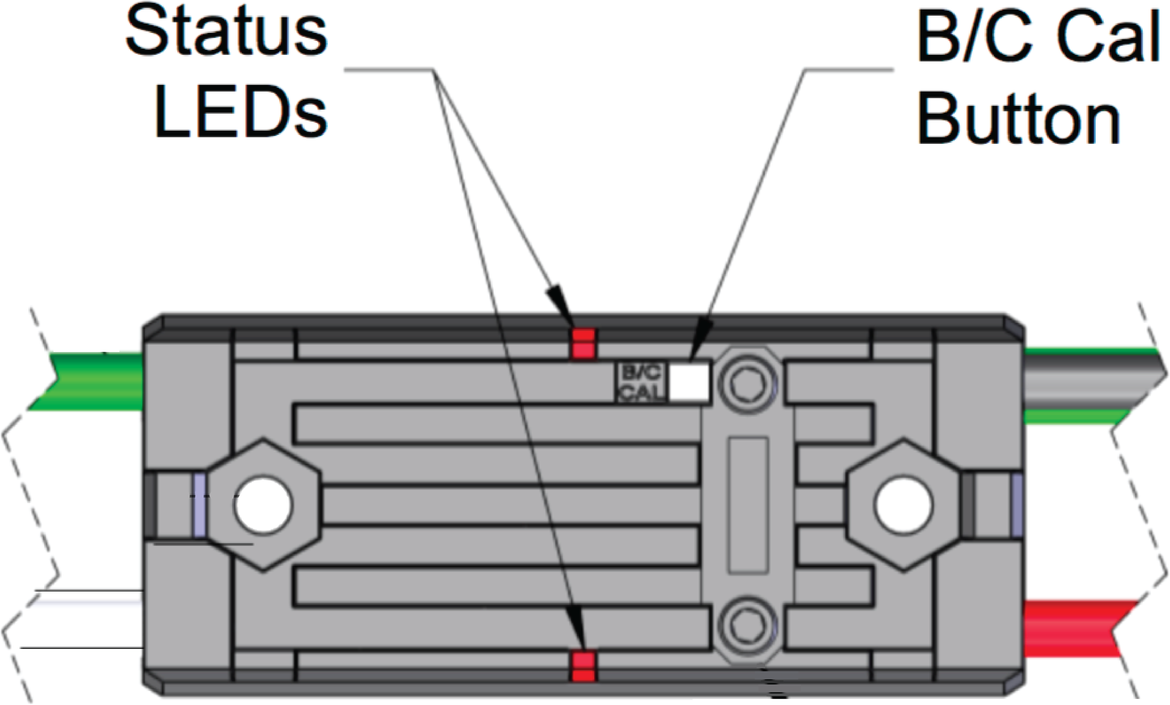
Status LEDs During Normal Operation
LEDs |
Colors |
Talon SRX State |
|---|---|---|
Both |
Blinking Green |
Forward throttle is applied. Blink rate is proportional to Duty Cycle. |
Both |
Blinking Red |
Reverse throttle is applied. Blink rate is proportional to Duty Cycle. |
None |
None |
No power is being applied to Talon SRX |
LEDs Alternate |
Off/Orange |
CAN bus detected, robot disabled |
LEDs Alternate |
Off/Slow Red |
CAN bus/PWM is not detected |
LEDs Alternate |
Off/Fast Red |
Fault Detected |
LEDs Alternate |
Red/Orange |
Damaged Hardware |
LEDs Strobe towards (M-) |
Off/Red |
Forward Limit Switch or Forward Soft Limit |
LEDs Strobe towards (M+) |
Off/Red |
Reverse Limit Switch or Reverse Soft Limit |
LED1 Only (closest to M+/V+) |
Green/Orange |
In Boot-loader |
LEDs Strobe towards (M+) |
Off/Orange |
Thermal Fault / Shutoff (Talon FX Only) |
Status LEDs During Calibration
Status LEDs Blink Code |
Talon SRX State |
|---|---|
Flashing Red/Green |
Calibration Mode |
Blinking Green |
Successful Calibration |
Blinking Red |
Failed Calibration |
B/C CAL Blink Codes
B/C CAL Button Color |
Talon SRX State |
|---|---|
Solid Red |
Brake Mode |
Off |
Coast Mode |
SPARK-MAX Motor Controller
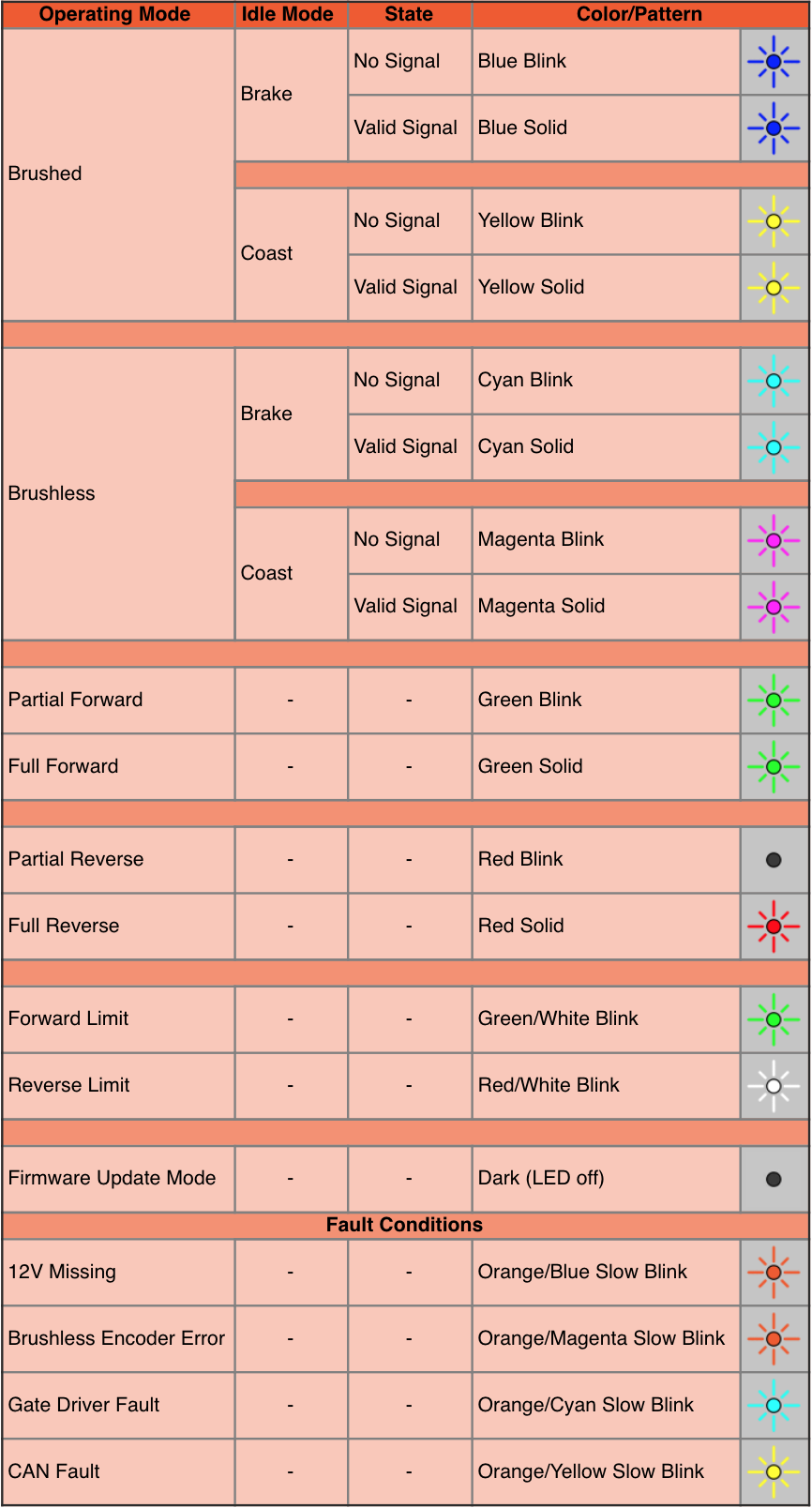
REV Robotics SPARK
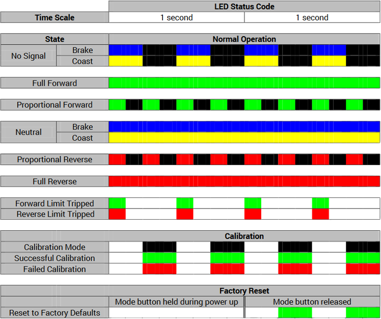
Victor-SP Motor Controller
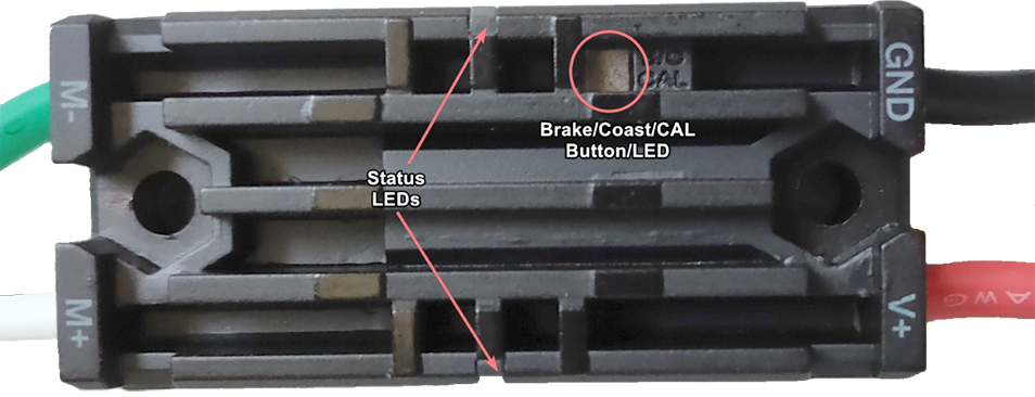
Brake/Coast/Cal Button/LED - Red if the controller is in brake mode, off if the controller is in coast mode
Status
Green |
Solid |
Full forward output |
Blinking |
Proportional to forward output voltage |
|
Red |
Solid |
Full reverse output |
Blinking |
Proportional to forward output voltage |
|
Orange |
Solid |
FRC robot disabled, PWM signal lost, or signal in deadband range (+/- 4% output) |
Red/Green |
Blinking |
Ready for calibration. Several green flashes indicates successful calibration, and red several times indicates unsuccessful calibration. |
Talon Motor Controller

Green |
Solid |
Full forward output |
Blinking |
Proportional to forward output voltage |
|
Red |
Solid |
Full reverse output |
Blinking |
Proportional to reverse output voltage |
|
Orange |
Solid |
No CAN devices are connected |
Blinking |
Disabled state, PWM signal lost, FRC robot disabled, or signal in deadband range (+/- 4% output) |
|
Off |
No input power to Talon |
|
Red/Green |
Flashing |
Ready for calibration. Several green flashes indicates successful calibration, and red several times indicates unsuccessful calibration. |
Victor888 Motor Controller

Green |
Solid |
Full forward output |
Blinking |
Successful calibration |
|
Red |
Solid |
Full reverse output |
Blinking |
Unsuccessful calibration |
|
Orange |
Solid |
Neutral/brake |
Red/Green |
Blinking |
Calibration mode |
Jaguar Motor Controller
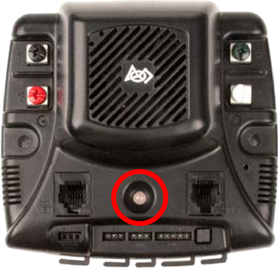
LED State |
Module Status |
|---|---|
Normal Operating Conditions |
|
Solid Yellow |
Neutral (speed set to 0) |
Fast Flashing Green |
Forward |
Fast Flashing Red |
Reverse |
Solid Green |
Full-speed forward |
Solid Red |
Full-speed reverse |
Fault Conditions |
|
Slow Flashing Yellow |
Loss of servo or Network link |
Fast Flashing Yellow |
Invalid CAN ID |
Slow Flashing Red |
Voltage, Temperature, or Limit Switch fault condition |
Slow Flashing Red and Yellow |
Current fault condition |
Calibration or CAN Conditions |
|
Flashing Red and Green |
Calibration mode active |
Flashing Red and Yellow |
Calibration mode failure |
Flashing Green and Yellow |
Calibration mode success |
Slow Flashing Green |
CAN ID assignment mode |
Fast Flashing Yellow |
Current CAN ID (count flashes to determine ID) |
Flashing Yellow |
CAN ID invalid (that is, Set to 0) awaiting valid ID assignment |
Digilent DMC-60
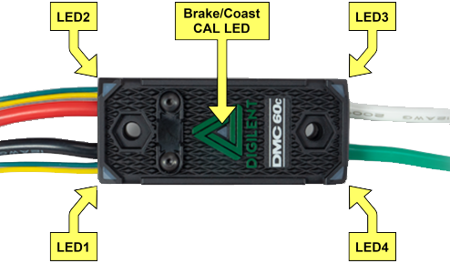
The DMC60C contains four RGB (Red, Green, and Blue) LEDs and one Brake/Coast CAL LED. The four RGB LEDs are located in the corners and are used to indicate status during normal operation, as well as when a fault occurs. The Brake/Coast CAL LED is located in the center of the triangle, which is located at the center of the housing, and is used to indicate the current Brake/Coast setting. When the center LED is off, the device is operating in coast mode. When the center LED is illuminated, the device is operating in brake mode. The Brake/Coast mode can be toggled by pressing down on the center of the triangle, and then releasing the button.
At power-on, the RGB LEDs illuminate Blue, continually getting brighter. This lasts for approximately five seconds. During this time, the motor controller will not respond to an input signal, nor will the output drivers be enabled. After the initial power-on has completed, the device begins normal operation and what gets displayed on the RGB LEDs is a function of the input signal being applied, as well as the current fault state. Assuming that no faults have occurred, the RGB LEDs function as follows:
PWM Signal Applied |
LED State |
|---|---|
No Input Signal or Invalid Input Pulse Width |
Alternate between top (LED1 and LED2) and bottom (LED3 and LED4) LEDs being illuminated Red and Off. |
Neutral Input Pulse Width |
All 4 LEDs illuminated Orange. |
Positive Input Pulse Width |
LEDs blink Green in a clockwise circular pattern (LED1 → LED2 → LED3 → LED4 → LED1). The LED update rate is proportional to the duty cycle of the output and increases with increased duty cycle. At 100% duty cycle, all 4 LEDs are illuminated Green. |
Negative Input Pulse Width |
LEDs blink Red in a counter-clockwise circular pattern (LED1 → LED4 → LED3 → LED2 → LED1). The LED update rate is proportional to the duty cycle of the output and increases with increased duty cycle. At 100% duty cycle, all 4 LEDs are illuminated Red. |
CAN Bus Control State |
LED State |
|---|---|
No Input Signal or CAN bus error detected |
Alternate between top (LED1 and LED2) and bottom (LED3 and LED4) LEDs being illuminated Red and Off. |
No CAN Control Frame received within the last 100ms or the last control frame specified modeNoDrive (Output Disabled) |
Alternate between top (LED1 and LED2) and bottom (LED3 and LED4) LEDs being illuminated Orange and Off. |
Valid CAN Control Frame received within the last 100ms. The specified control mode resulted in a Neutral Duty Cycle being applied to Motor Output |
All 4 LEDs illuminated solid Orange. |
Valid CAN Control Frame received within the last 100ms. The specified control mode resulted in a Positive Duty Cycle being Motor Output |
LEDs blink Green in a clockwise circular pattern (LED1 → LED2 → LED3 → LED4 → LED1). The LED update rate is proportional to the duty cycle of the output and increases with increased duty cycle. At 100% duty cycle, all 4 LEDs are illuminated Green. |
Valid CAN Control Frame received within the last 100ms. The specified control mode resulted in a Negative Duty Cycle being Motor Output |
LEDs blink Red in a counter-clockwise circular pattern (LED1 → LED4 → LED3 → LED2 → LED1). The LED update rate is proportional to the duty cycle of the output and increases with increased duty cycle. At 100% duty cycle, all 4 LEDs are illuminated Red. |
Fault Color Indicators
When a fault condition is detected, the output duty cycle is reduced to 0% and a fault is signaled. The output then remains disabled for 3 seconds. During this time the onboard LEDs (LED1-4) are used to indicate the fault condition. The fault condition is indicated by toggling between the top (LED1 and LED2) and bottom (LED3 and LED4) LEDs being illuminated Red and off. The color of the bottom LEDs depends on which faults are presently active. The table below describes how the color of the bottom LEDs maps to the presently active faults.
Color |
Over Temperature |
Under Voltage |
|---|---|---|
Green |
On |
Off |
Blue |
Off |
On |
Cyan / Aqua |
On |
On |
Break/Coast Mode
When the center LED is off the device is operating in coast mode. When the center LED is illuminated the device is operating in brake mode. The Brake/Coast mode can be toggled by pressing down on the center of the triangle and then releasing the button.
Venom Motor Controller
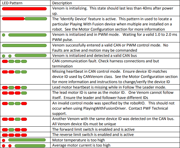
Mindsensors SD540B (PWM)
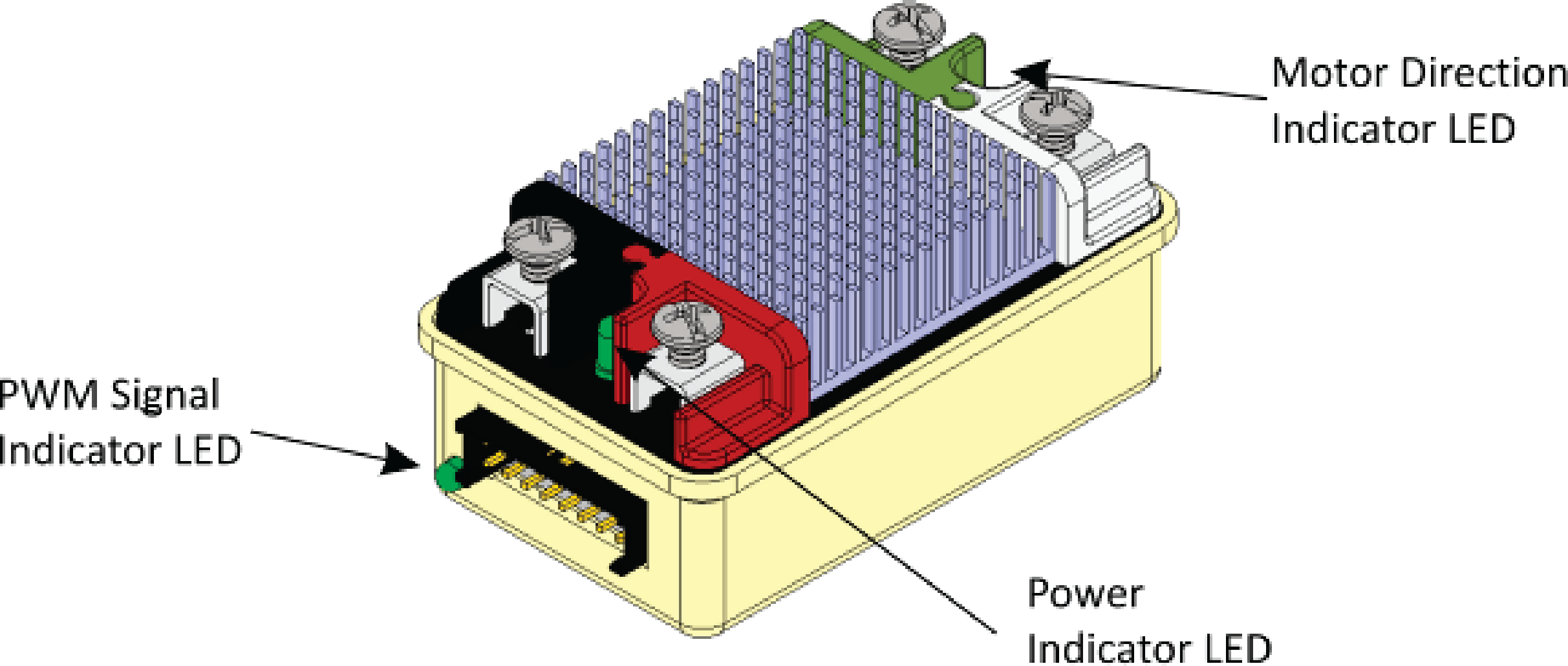
Power LED |
Off |
Power is not supplied |
Red |
Power is supplied |
|
Motor LED |
Red |
Forward direction |
Green |
Reverse direction |
|
PWM Signal LED |
Red |
No valid PWM signal is detected |
Green |
Valid PWM signal is detected |
Mindsensors SD540C (CAN Bus)
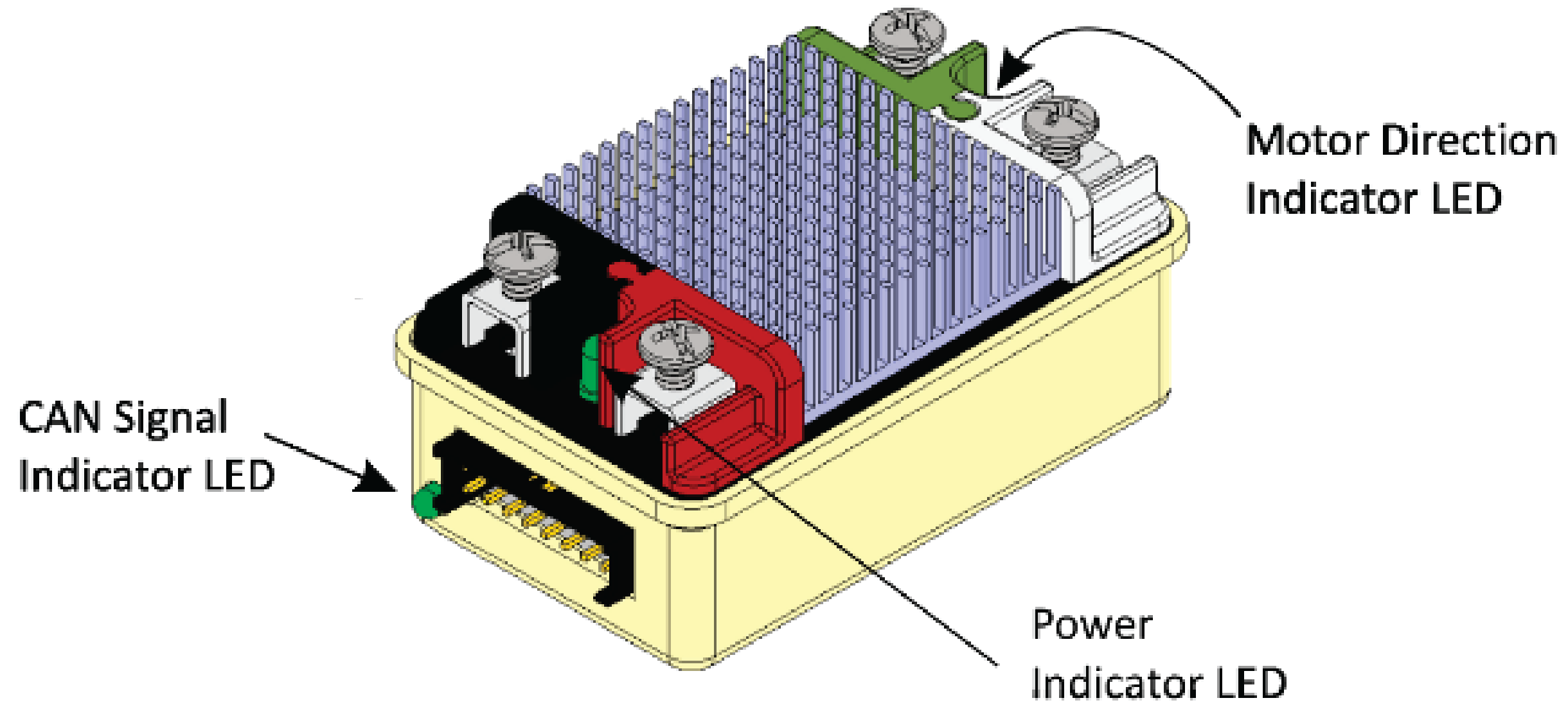
Power LED |
Off |
Power is not supplied |
Red |
Power is supplied |
|
Motor LED |
Red |
Forward direction |
Green |
Reverse direction |
|
CAN Signal LED |
Blinking quickly |
No CAN devices are connected |
Off |
Connected to the roboRIO and the driver station is open |
REV Robotics Servo Power Module
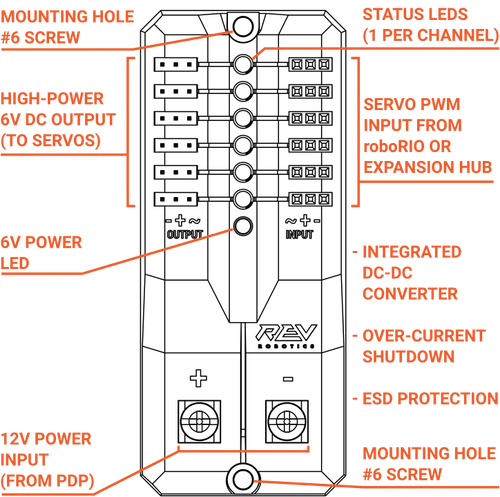
Status LEDs
Each channel has a corresponding status LED that will indicate the sensed state of the connected PWM signal. The table below describes each state’s corresponding LED pattern.
State |
Pattern |
|---|---|
No Signal |
Blinking Amber |
Left/Reverse Signal |
Solid Red |
Center/Neutral Signal |
Solid Amber |
Right/Forward Signal |
Solid Green |
6V Power LED off, dim or flickering with power applied = Over-current shutdown
Spike relay configured as a motor, light, or solenoid switch
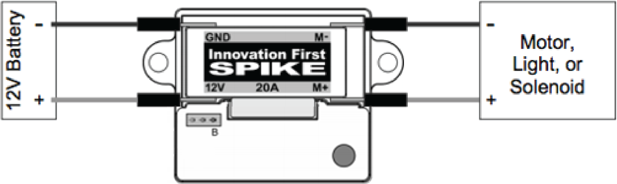
Inputs |
Outputs |
Indicator |
Motor Function |
||
Forward (White) |
Reverse (Red) |
M+ |
M- |
||
Off |
Off |
GND |
GND |
Orange |
Off/Brake Condition (default) |
On |
Off |
+12v |
GND |
Green |
Motor rotates in one direction |
Off |
On |
GND |
+12v |
Red |
Motor rotates in opposite direction |
On |
On |
+12v |
+12v |
Off |
Off/Brake Condition |
Note
‘Brake Condition’ refers to the dynamic stopping of the motor due to the shorting of the motor inputs. This condition is not optional when going to an off state.
Spike relay configured as for one or two solenoids

Inputs |
Outputs |
Indicator |
Motor Function |
||
Forward (White) |
Reverse (Red) |
M+ |
M- |
||
Off |
Off |
GND |
GND |
Orange |
Both Solenoids Off (default) |
On |
Off |
+12v |
GND |
Green |
Solenoid connected to M+ is ON |
Off |
On |
GND |
+12v |
Red |
Solenoid connected to M- is ON |
On |
On |
+12v |
+12v |
Off |
Both Solenoids ON |
Robot Preemptive Troubleshooting
Note
In FIRST® Robotics Competition, robots take a lot of stress while driving around the field. It is important to make sure that connections are tight, parts are bolted securely in place and that everything is mounted so that a robot bouncing around the field does not break.
Check Battery Connections
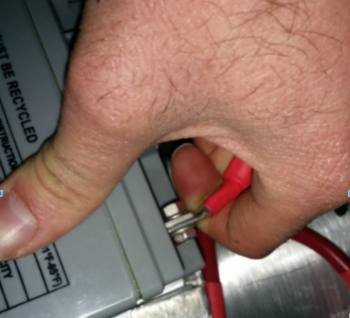
The tape that should be covering the battery connection in these examples has been removed to illustrate what is going on. On your robots, the connections should be covered.
Wiggle battery harness connector. Often these are loose because the screws loosen, or sometimes the crimp is not completely closed. You will only catch the really bad ones though because often the electrical tape stiffens the connection to a point where it feels stiff. Using a voltmeter or Battery Beak will help with this.
Apply considerable force onto the battery cable at 90 degrees to try to move the direction of the cable leaving the battery, if successful the connection was not tight enough to begin with and it should be redone. This article has more detailed battery information.
Securing the Battery to the Robot
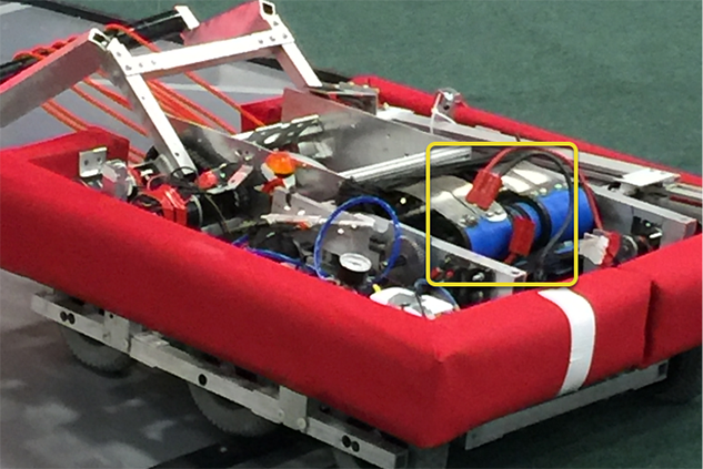
In almost every event we see at least one robot where a not properly secured battery connector (the large Anderson) comes apart and disconnects power from the robot. This has happened in championship matches on the Einstein and everywhere else. Its an easy to ensure that this doesn’t happen to you by securing the two connectors by wrapping a tie wrap around the connection. 10 or 12 tie wraps for the piece of mind during an event is not a high price to pay to guarantee that you will not have the problem of this robot from an actual event after a bumpy ride over a defense. Also, secure your battery to the chassis with hook and loop tape or another method, especially in games with rough defense, obstacles or climbing.
Securing the Battery Connector & Main Power Leads
A loose robot-side battery connector (the large Anderson SB) can allow the main power leads to be tugged when the battery is replaced. If the main power leads are loose, that “tug” can get all the way back to the crimp lugs attached to the 120 Amp Circuit Breaker or Power Distribution Panel (PDP), bend the lug, and over time cause the lug end to break from fatigue. Putting a couple tie wraps attaching the main power leads to the chassis and bolting down the robot-side battery connector can prevent this, as well as make it easier to connect the battery.
Main Breaker (120 Amp Circuit Breaker)
Note
Ensure nuts are tightened firmly and the breaker is attached to a rigid element.
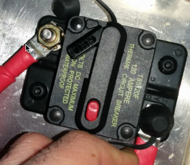
Apply a strong twisting force to try to rotate the crimped lug. If the lug rotates then the nut is not tight enough. After tightening the nut, retest by once again trying to rotate the lug.
The original nut has a star locking feature, which can wear out over time: these may require checking every few matches, especially if your robot-side battery connector is not attached to the chassis.
The nut is normally a relatively uncommon 1/4-28 thread: ensure this is correct if the nut is replaced.
Because the metal stud is just molded into the case, every once in awhile you may break off the stud. Don’t stress, just replace the assembly.
When subjected to multiple competition seasons, the Main Breaker is susceptible to fatigue damage from vibration and use, and can start opening under impact. Each time the thermal fuse function is triggered, it can become progressively easier to trip. Many veteran teams start each season with a fresh main breaker, and carry spares.
Power Distribution Panel (PDP)
Make sure that split washers were placed under the PDP screws, but it is not easy to visually confirm, and sometimes you can’t. You can check by removing the case. Also if you squeeze the red and black wires together, sometimes you can catch the really lose connections.
Tug Testing
The Weidmuller contacts for power, compressor output, roboRIO power connector, and radio power are important to verify by tugging on the connections as shown. Make sure that none of the connections pull out.
Look for possible or impending shorts with Weidmuller connections that are close to each other, and have too-long wire-lead lengths (wires that are stripped extra long).
Spade connectors can also fail due to improper crimps, so tug-test those as well.
Blade Fuses
Be sure to place the 20A fuse (yellow) on the left and the 10A fuse (red) on the right.

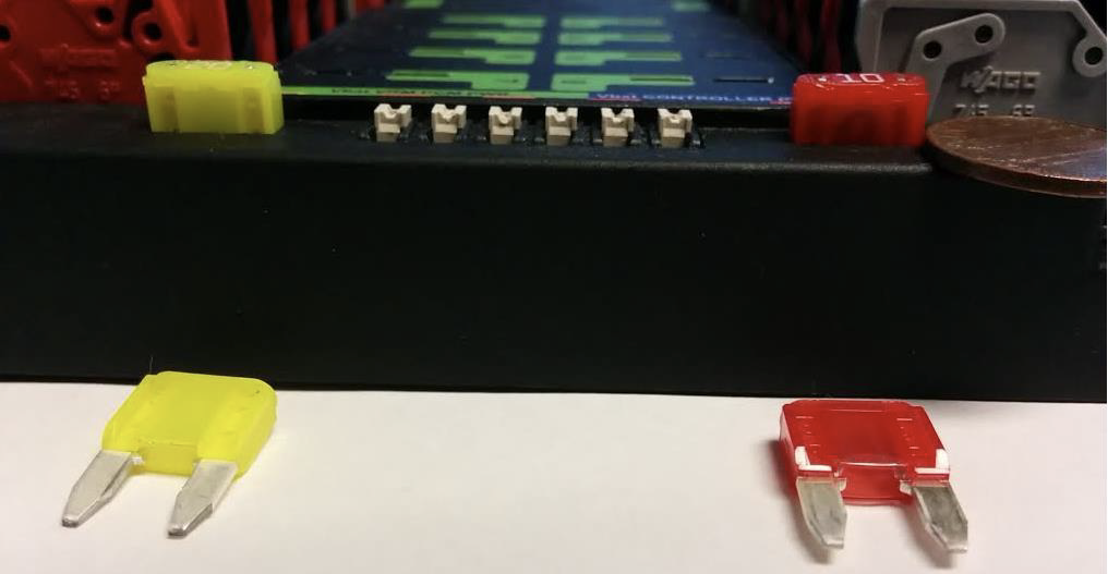
Warning
Take care to ensure fuses are fully seated into the fuse holders. The fuses should descend at least as far as the figure below (different brand fuses have different lead lengths). It should be nearly impossible to remove the fuse with bare hands (without the use of pliers). If this is not properly done, the robot/radio may exhibit intermittent connectivity issues.
If you can remove the blade fuses by hand then they are not in completely. Make sure that they are completely seated in the PDP so that they don’t pop out during robot operation.
roboRIO swarf
Swarf is fine chips or filings of stone, metal, or other material produced by a machining operation. Often modifications must be made to a robot while the control system parts are in place. The circuit board for the roboRIO is conformally coated, but that doesn’t absolutely guarantee that metal chips won’t short out traces or components inside the case. In this case, you must exercise care in making sure that none of the chips end up in the roboRIO or any of the other components. In particular, the exposed 3 pin headers are a place where chips can enter the case. A quick sweep through each of the four sides with a flashlight is usually sufficient to find the really bad areas of infiltration.
Radio Barrel Jack
Make sure the correct barrel jack is used, not one that is too small and falls out for no reason. This isn’t common, but ask an FTA and every once in awhile a team will use some random barrel jack that is not sized correctly, and it falls out in a match on first contact.
Ethernet Cable
If the RIO to radio ethernet cable is missing the clip that locks the connector in, get another cable. This is a common problem that will happen several times in every competition. Make sure that your cables are secure. The clip often breaks off, especially when pulling it through a tight path, it snags on something then breaks.
Loose Cables
Cables must be tightened down, particularly the radio power and ethernet cable. The radio power cables don’t have a lot of friction force and will fall out (even if it is the correct barrel) if the weight of the cable-slack is allowed to swing freely.
Ethernet cable is also pretty heavy, if it’s allowed to swing freely, the plastic clip may not be enough to hold the ethernet pin connectors in circuit.
Reproducing Problems in the Pit
Beyond the normal shaking of cables whilst the robot is powered and tethered, it is suggested that one side of the robot be picked up and dropped. Driving on the field, especially against defenders, will often be very violent, and this helps makes sure nothing falls out. It is better for the robot to fail in the pits rather than in the middle of a match.
When doing this test it’s important to be ethernet tethered and not USB tethered, otherwise you are not testing all of the critical paths.
Check Firmware and Versions
Robot inspectors do this, but you should do it as well, it helps robot inspectors out and they appreciate it. And it guarantees that you are running with the most recent, bug fixed code. You wouldn’t want to lose a match because of an out of date piece of control system software on your robot.
Driver Station Checks
We often see problems with the Drivers Station. You should:
ALWAYS bring the laptop power cable to the field, it doesn’t matter how good the battery is, you are allowed to plug in at the field.
Check the power and sleep settings, turn off sleep and hibernate, screen savers, etc.
Turn off power management for USB devices (dev manager)
Turn off power management for ethernet ports (dev manager)
Turn off windows defender
Turn off firewall
Close all apps except for DS/Dashboard when out on the field.
Verify that there is nothing unnecessary running in the application tray in the start menu (bottom right side)
Handy Tools
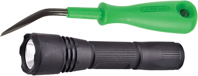
There never seems to be enough light inside robots, at least not enough to scrutinize the critical connection points, so consider using a handheld LED flashlight to inspect the connections on your robot. They’re available from home depot or any hardware/automotive store.
A WAGO tool is nice tool for redoing Weidmuller connections with stranded wires. Often I’ll do one to show the team, and then have them do the rest using the WAGO tool to press down the white-plunger while they insert the stranded wire. The angle of the WAGO tool makes this particularly helpful.
Robot Battery Basics
The power supply for an FRC® robot is a single 12V 18Ah SLA (Sealed Lead Acid) non-spillable battery, capable of briefly supplying over 180A and arcing over 500A when fully charged. The Robot Battery assembly includes the COTS battery, lead cables with contacts, and Anderson SB connector. Teams are encouraged to have multiple Robot Batteries.
COTS Battery
The Robot Rules in the Game Manual specify a Commercial Off The Shelf [COTS] non-spillable sealed lead acid battery meeting specific criteria, and gives examples of legal part numbers from a variety of vendors.
Battery Safety & Handling
A healthy battery is always “On” and the terminals are always energized. If the polarities short together - for example, a wrench or aerosol can falls and bridges the gap between two bare terminals - all the stored energy will be released in a dangerous arc. This risk drives a wide range of best practices, such as covering terminals in storage, only uncovering and working on one terminal or polarity at a time, keeping SB contacts fully inserted in connectors, etc.
Do *NOT* carry a battery assembly by the cables, and always avoid pulling by them. Pulling on batteries by the cables will begin to damage the lugs, tabs, and the internal connection of the tab. Over time, fatigue damage can add up until the the entire tab tears out of the housing! Even if it isn’t clearly broken, internal fatigue damage can increase the battery internal resistance, prematurely wearing out the battery. The battery will not be able to provide the same amount of current with increased internal resistance or if the connectors are loose.
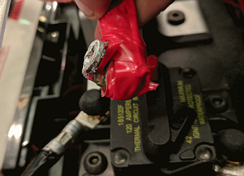
Dropping the batteries can bend the internal plates and cause performance issues, create bulges, or even crack the battery case open. While most FRC batteries use Absorbent Glass Mat [AGM] or Gel technology for safety and performance, when a cell is punctured it may still leak a small amount of battery acid. This is one of the reasons FIRST recommends teams have a battery spill kit available.
Finally, certain older battery chargers without “maintenance mode” features can overcharge the battery, resulting in boiling off some of the battery acid.
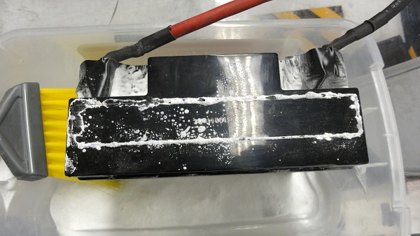
Damaged batteries should be safely disposed of as soon as possible. All retailers that sell large SLA batteries, like car batteries, should be able to dispose of it for you. They may charge a small fee, or provide a small “core charge refund”, depending on your state law.
Danger
DO NOT attempt to “repair” damaged or non-functional batteries.
Battery Construction & Tools
Battery Leads
Battery leads must be copper, minimum size (cross section) 6 AWG (16mm2, 7 SWG) and maximum length 12”, color coded for polarity, with an Anderson SB connector. Standard 6AWG copper leads with Pink/Red SB50 battery leads often come in the Kit of Parts and are sold by FRC vendors.
Lead Cables
Tinned, annealed, or coated copper is allowed. Do not use CCA (copper clad aluminum), aluminum, or other non-copper base metal. The conductor metal is normally printed on the outside of the insulation with the other cable ratings.
Wire size 6AWG is sufficient for almost all robots and fits standard SB50 contacts. A small number of teams adopt larger wire sizes for marginal performance benefits.
Higher strand count wire (sometimes sold as “Flex” or “welding wire”) has a smaller bend radius, which makes it easier to route, and a higher fatigue limit. There is no strand count requirement, but 84/25 (84 strand “flex” hookup wire) and 259/30 (259 strand “welding wire”) will both be much easier to work with than 19/0.0372 (19 strand hookup wire).
The insulation must be color-coded per the Game Manual: as of 2021, the +12Vdc wire must be red, white, brown, yellow, or black w/stripe and the ground wire (return wire) must be black or blue. There is no explicit insulation temperature rating requirement, but any blackened or damaged insulation means the wire needs to be replaced: off hand, 105C is plenty and lower will work for almost all robots. There is no insulation voltage rating requirement, lower is better for thinner insulation.
SB Connector
The Anderson SB Connector may be the standard Pink/Red SB50, or another Anderson SB connector. Teams are STRONGLY recommended to use the Pink/Red SB50 for interoperability: the other colors and sizes of housings will not intermate, and you will be unable to borrow batteries or chargers.
Follow manufacturer’s instructions to crimp contacts and assemble the leads into Anderson SB connectors. A small flathead screwdriver can help to insert the contacts (push on the contact, not on the wire insulation), or it can help to disengage the internal latch if the contact is in the wrong slot or upside down.
Battery Lugs
Compression lugs (“crimp lugs”) for #10 bolt (or M5) battery tabs (~0.2” or ~5mm hole diameter) are available online and through electrical supply houses, sold by the accepted wire sizes in AWG (or mm2) and post diameter (“bolt size”, “hole diameter”). Higher end vendors will also distinguish between Standard (~19) and Flex (>80) strand counts in their lug catalogs. Some vendors also offer right angle lugs, in addition to more common straight styles. Follow manufacturer’s instructions to crimp the lugs.
Screw terminal lugs are legal, but not recommended. If using screw terminal lugs, use the correct tip size screwdriver to tighten the terminal. Check the terminal tightness frequently because they may loosen over time.
Battery Lead Lug To Post Connection
A #10 or M5 nut & bolt connect the battery lead lug to the battery tab.
Warning
The lug and tab must directly contact, copper to copper: do not put a washer of any kind separating them.
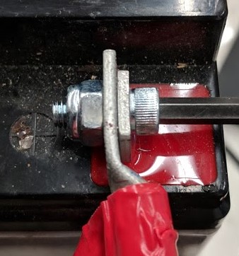
Some batteries come with tab bolts in the package: they may be used, or replaced with stronger alloy steel bolts. It is a good idea to add a functional lock washer, such as a #10 star washer or a nordlock washer system, in addition to a nylon locking (“nylock”) nut. Only use one style of lock washer in each connection. Even if the manufacturer provides split ring lock washers in the package, you are not required to use them.
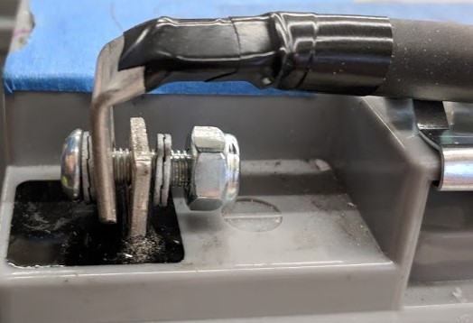
These connections must be very tight for reliability. Any movement of the lug while in operation may interrupt robot power, resulting in robot reboots and field disconnections lasting 30 seconds or more.
This connection must also be completely covered for electrical safety; electrical tape will work, but heatshrink that fits over the entire connection is recommended. High shrink ratios (minimum 3:1, recommend 4:1) will make it easier to apply the heatshrink. Adhesive lined heat shrink is allowed. Be sure all the copper is covered! Heat shrink must be “touched up” with electrical tape if some copper shows.
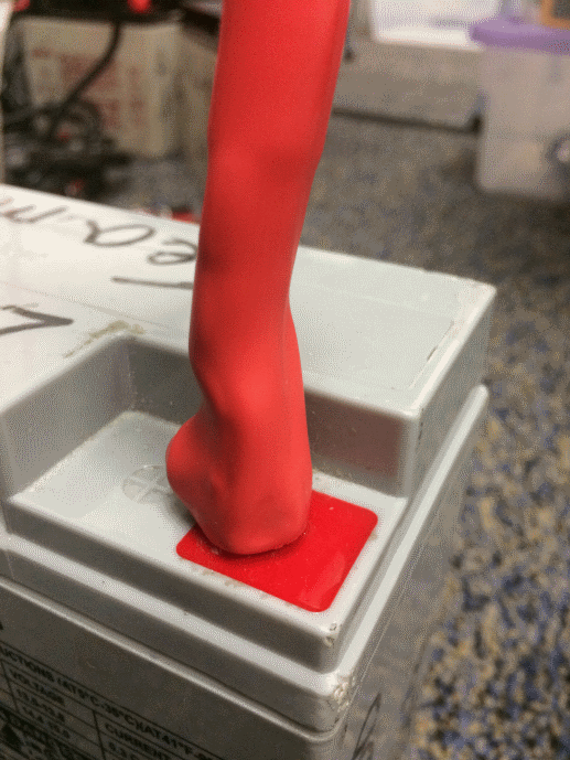
Battery Chargers
There are many good COTS “smart” battery chargers designed for 12V SLA batteries, rated for 6A or less per battery, with ‘maintenance mode’ features. Chargers rated over 6A are not allowed in FRC pits.
Chargers used at competition are required to use Anderson SB connectors. Attaching a COTS SB connector battery lead to the charger leads using appropriately sized wire nuts or screw terminals is fast and simple (be sure to cover any exposed copper with heat shrink or electrical tape). SB Connector Contacts are also available for smaller wire sizes, if the team has crimping capability.
Warning
After attaching the SB, double check the charger polarities with a multimeter before plugging in the first battery.
Some FRC vendors sell chargers with red SB50 connectors pre-attached.
Battery Evaluation Tools
Battery Charger
If your battery charger has Maintenance Mode indicator, such as a GREEN LED, you can use that indicator to tell you whether you are READY. Some chargers will cycle between “CHARGING” and “READY” periodically. This is a “maintenance” behavior, sometimes associated with the battery cooling off and being able to accept more charge.
Driver Station Display and Log
When the robot is plugged in and connected to the driver station laptop, the battery voltage is displayed on the NI Driver Station software.
After you finish a driving session, you can review the battery voltage in the Log Viewer.
Hand-held Voltmeter or Multimeter
A voltage reading from probes on the SB connector of a disconnected battery will give you a snapshot of what the Voc (Voltage open circuit, or “float voltage”) is in the “Unloaded” state. In general the Voc is not a recommended method for understanding battery health: the open circuit voltage is not as useful as the combination of internal resistance and voltages at specific loads provided by a Load Tester (or Battery Analyzer).
Load Tester
A battery load tester can be used as a quick way to determine the detailed readiness of a battery. It may provide information like: open-load voltage, voltage under load, internal resistance, and state of charge. These metrics can be used to quickly confirm that a battery is ready for a match and even help to identify some long term problems with the battery.
Ideal internal resistance should be less than 0.015 Ohms. The manufacturer specification for most batteries is 0.011 Ohms. If a battery gets higher than 0.020 Ohms it is a good idea to consider not using that battery for competition matches.
If a battery shows significantly lower voltages at the higher test current loads, it may not be done charging, or it may need to be retired.
Understanding Battery Voltages
A “12V battery” is anything but 12.0V.
Fully charged, a battery can be anywhere from 12.7 to 13.5 volts open circuit (Voc). Open circuit voltage is measured with nothing connected.
Once a load (like a robot) is connected, and any amount of current is flowing, the battery voltage will drop. So if you check a battery with a Voltmeter, and it reads 13.2, and then connect it to your robot and power on, it will read lower, maybe 12.9 on the Driver Station display. Those numbers will vary with every battery and specific robot, see Characterization below. Once your robot starts running, it will pull more current, and the voltage will drop further.
Batteries reading 12.5V on an idle robot should be swapped and charged before a match. Always swap the batteries before the robot starts reaching brownout safety thresholds (dwelling at low voltages on the Driver Station display), as frequently entering low voltage ranges risks permanent battery damage; this behavior can happen at a variety of Voc states depending on battery health, battery manufacturer, and robot design. The battery State of Charge should be kept over 50% for battery longevity.
Battery voltage and current also depends on temperature: cool batteries are happy batteries.
Battery Characterization
A battery analyzer can be used to give a detailed inspection and comparison of battery performance.
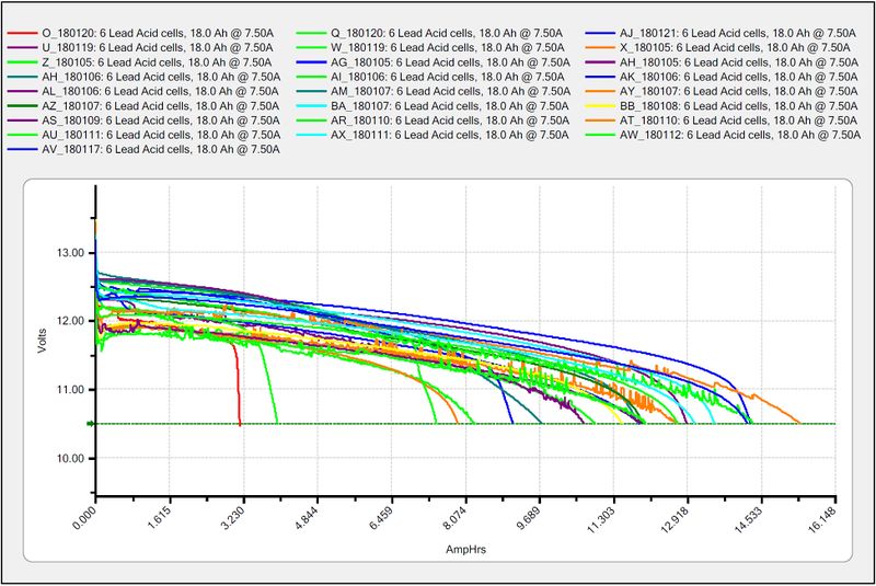
It will provide graphs of battery performance over time. This test takes significant time (roughly two hours) so it is less suited to testing during competition. It is recommended to run this test on each battery every year to monitor and track its performance. This will determine how it should be used: matches, practice, testing, or disposed of.
At the standard 7.5 amps test load, competition batteries should have at least a 11.5 amp hour rating. Anything less than that should only be used for practice or other less demanding use cases.
Battery Longevity
A battery is rated for about 1200 normal charge/recharge cycles. The high currents required for an FRC match reduce that lifespan to about 400 cycles. These cycles are intended to be relatively low discharge, from around 13.5 down to 12 or 12.5 volts. Deep cycling the battery (running it all the way down) will damage it.
Batteries last the longest if they are kept fully charged when not it use, either by charging regularly or by use of a maintenance charger. Batteries drop roughly 0.1V every month of non-use.
Batteries need to be kept away from both extreme heat and cold. This generally means storing the batteries in a climate controlled area: a classroom closet is usually fine, a parking lot shipping container is more risky.
Battery Best Practices
Only use a charged battery for competition matches. If you are in a situation where you have run out of charged batteries, please ask a veteran team for help! Nobody wants to see a robot dead on the field (brownout) due to a bad or uncharged battery.
Teams are strongly recommended to use properly rated tools and stringent quality control practices for crimping processes (ask local veteran teams or a commercial electrician for help), or use vendor-made Battery Leads.
Wait for batteries to cool after the match before recharging: the case should not be warm to the touch, fifteen minutes is usually plenty.
Teams should consider purchasing several new batteries each year to help keep their batteries fresh. Elimination matches can require many batteries and there may not be enough time to recharge.
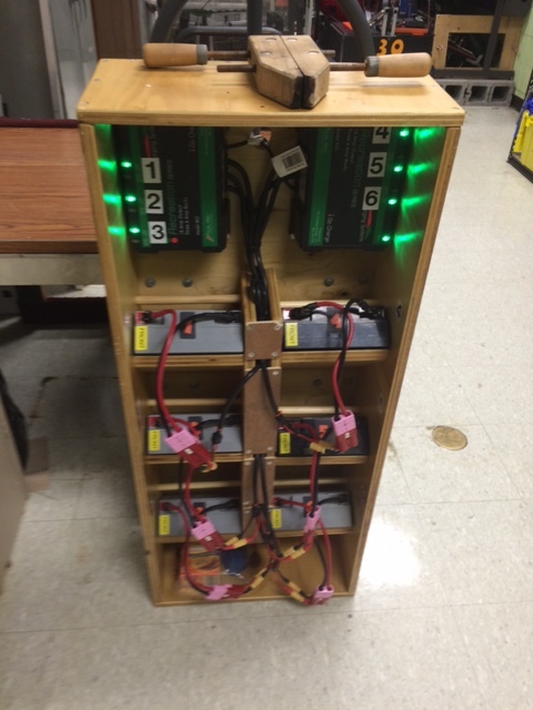
A multi bank battery charger allows you to charge more than one battery at a time. Many teams build a robot cart for their batteries and chargers allowing for easy transport and storage.
It is a good idea to permanently identify each battery with at least: team number, year, and a unique identifier.
Teams may also want to use something removeable (stickers, labeling machine etc.) to identify what that battery should be used for based on its performance data and when the last analyzer test was run.
Using battery flags (a piece of plastic placed in the battery connector) is a common way to indicate that a battery has been charged. Battery flags can also be easily 3D printed.
Handles for SB50 contacts can be purchased or 3D printed to help avoid pulling on the leads while connecting or disconnecting batteries. Do not use these handles to carry the weight of the battery.

Some teams sew battery carrying straps from old seatbelts or other flat nylon that fit around the battery to help prevent carrying by leads.
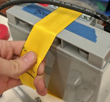
Cable tie edge clips can be used with 90 degree crimp lugs to strain relieve battery leads.
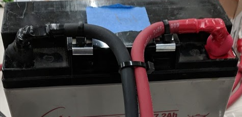
Hardware Tutorials
Note
The pages in this section of the documentation contain media which is only viewable from the web version of the documentation
Motors for Robotics Applications
One of the most important design decisions that teams have to deal with is selecting and designing the motor driven systems on their robot. So often the incorrect motor is chosen for a particular design yielding reduced performance and, sometimes even worse, motors failing from excessive current draw. In this series of videos, WPI Professor Ken Stafford walks through how motors work, how to design systems to operate at maximum performance, and a sample design for a robot system.
Sensing and Sensors
Without sensors and sensing robots are really radio controlled vehicles. Sensors allow the robots to understand the internal operation of the robots mechanical systems as well as the ability to interact with the environment around the robot. In these videos, WPI Professor Craig Putnam describes a number of classes of sensors, how they are used, and provides guidance on what sensors are best for your applications.
Pneumatics
Pneumatics is an often underused actuation device that can be used on robots. There are many advantages to pneumatics over using motors. In this video Professor Ken Stafford describes the characteristics of pneumatics, applications with robots, and calculating the right sized system for an application.
Power Transmission
Hand in hand with choosing the correct motors for an application is transmitting that motor power to the place it’s needed. Using gears or chains and sprockets are two effective ways of matching the motor power to the application being driven. In this video, WPI Robotics Engineering PhD student Michael Delph talks about power transmission, including choosing correct gear or chain and sprocket ratios to get the the maximum performance from your robot design.
Sensors
Sensor Overview - Hardware
Note
This section covers sensor hardware, not the use of sensors in code. For a software sensor guide, see Sensor Overview - Software.
In order to be effective, it is often vital for robots to be able to gather information about their surroundings. Devices that provide feedback to the robot on the state of its environment are called “sensors.” There are a large variety of sensors available to FRC® teams, for measuring everything from on-field positioning to robot orientation to motor/mechanism positioning. Making use of sensors is an absolutely crucial skill for on-field success; while most FRC games do have tasks that can be accomplished by a “blind” robot, the best robots rely heavily on sensors to accomplish game tasks as quickly and reliably as possible.
Additionally, sensors can be extremely important for robot safety - many robot mechanisms are capable of breaking themselves if used incorrectly. Sensors provide a safeguard against this, allowing robots to, for example, disable a motor if a mechanism is against a hard-stop.
Types of Sensors
Sensors used in FRC can be generally categorized in two different ways: by function, and by communication protocol. The former categorization is relevant for robot design; the latter for wiring and programming.
Sensors by Function
Sensors can provide feedback on a variety of different aspects of the robot’s state. Sensor functions common to FRC include:
-
Mechanical proximity switches (“limit switches”)
Magnetic proximity switches
Inductive proximity switches
Photoelectric proximity switches
Distance sensors
Shaft rotation sensors
Sensors by Communication Protocol
In order for a sensor to be useful, it must be able to “talk” to the roboRIO. There are several main methods by which sensors can communicate their readings to the roboRIO:
In general, support for sensors that communicate via analog and digital inputs is straightforward, while communication over serial bus can be more complicated.
Analog Inputs - Hardware
Note
This section covers analog input hardware. For a software guide to analog inputs, see Analog Inputs - Software.
An analog signal is a signal whose value can lie anywhere in a continuous interval. This lies in stark contrast to a digital signal, which can take only one of several discrete values. The roboRIO’s analog input ports allow the measurement of analog signals with values from 0V to 5V.
In practice, there is no way to measure a “true” analog signal with a digital device such as a computer (like the roboRIO). Accordingly, the analog inputs are actually measured as a 12-bit digital signal - however, this is quite a high resolution 1.
Analog inputs are typically (but not always!) used for sensors whose measurements vary continuously over a range, such as ultrasonic rangefinders and potentiometers, as they can communicate by outputting a voltage proportional to their measurements.
Connecting to roboRIO analog input ports
Note
An additional four analog inputs are available via the “MXP” expansion port. To use these, a breakout board of some sort that connects to the MXP is needed.
Warning
Always consult the technical specifications of the sensor you are using before wiring the sensor, to ensure that the correct wire is being connected to each pin. Failure to do so can result in damage to the sensor or the RIO.
Warning
Never directly connect the power pin to the ground pin on any port on the roboRIO! This will trigger protection features on the roboRIO and may result in unexpected behavior.

The roboRIO has 4 built-in analog input ports (numbered 0-3), as seen in the image above. Each port has three pins - signal (“S”), power (“V”), and ground (“⏚”). The “power” and “ground” pins are used to power the peripheral sensors that connect to the analog input ports - there is a constant 5V potential difference between the “power” and the “ground” pins 2. The signal pin is the pin on which the signal is actually measured.
Connecting a sensor to a single analog input port
Note
Some sensors (such as potentiometers) may have interchangeable power and ground connections.
Most sensors that connect to analog input ports will have three wires - signal, power, and ground - corresponding precisely to the three pins of the analog input ports. They should be connected accordingly.

Connecting a sensor to multiple analog input ports
Some sensors may need to connect to multiple analog input ports in order to function. In general, these sensors will only ever require a single power and a single ground pin - only the signal pin of the additional port(s) will be needed. The image below is shows an analog accelerometer that requires three digital input ports, but similar wiring can be used for analog sensors requiring two analog input ports.

Footnotes
- 1
A 12-bit resolution yields \(2^{12}\), or 4096 different values. For a 5V range, that’s an effective resolution of approximately 1.2 mV, or .0012V. The actual accuracy specification is plus-or-minus 50mV, so the discretization is not the limiting factor in the measurement accuracy.
- 2
All power pins are actually connected to a single rail, as are all ground pins - there is no need to use the power/ground pins corresponding to a given signal pin.
Analog Potentiometers - Hardware
Note
This section covers analog potentiometer hardware. For a software guide to analog potentiometers, see Analog Potentiometers - Software.
Warning
Potentiometers generally have a mechanically-limited travel range. Users should be careful that their mechanisms do not turn their potentiometers past their maximum travel, as this will damage or destroy the potentiometer.
Apart from quadrature encoders, another common way of measuring rotation on FRC® robots is with analog potentiometers. A potentiometer is simply a variable resistor - as the shaft of the potentiometer turns, the resistance changes (usually linearly). Placing this resistor in a voltage divider allows the user to easily measure the resistance by measuring the voltage across the potentiometer, which can then be used to calculate the rotational position of the shaft.
Wiring an analog potentiometer
As suggested by the names, analog potentiometers connect to the roboRIO’s analog input ports. To understand how exactly to wire potentiometers, however, it is important to understand their internal circuitry.

The picture above on the left shows a typical potentiometer. There are three pins, just as there are on the RIO’s analog inputs. The middle pin is the signal pin, while the outer pins can both be either power or ground.
As mentioned before, a potentiometer is a voltage divider, as shown in the circuit diagram on the right. As the potentiometer shaft turns, the resistances R1 and R2 change; however, their sum remains constant 1. Thus, the voltage across the entire potentiometer remains constant (for the roboRIO, this would be 5 volts), but the voltage between the signal pin and either the voltage or ground pin varies linearly as the shaft turns.
Since the circuit is symmetric, it is reversible - this allows the user to choose at which end of the travel the measured voltage is zero, and at which end it is 5 volts. To reverse the directionality of the sensor, it can simply be wired backwards! Be sure to check the directionality of your potentiometer with a multimeter to be sure it is in the desired orientation before soldering your wires to the contacts.
Absolute encoders

An “absolute encoder” is an encoder that measures the absolute position of the encoder shaft, rather than the incremental movement (as a quadrature encoder) does. In this respect, absolute encoders are more similar to potentiometers than to incremental encoders. Many absolute encoders offer a simple analog output - these can be used exactly in the same way as a potentiometer, except their wiring is not generally reversible. Absolute encoders have the advantage of lacking a hard travel limit - the signal will simply reset when the shaft crosses the zero point. The analog potentiometer pictured above can be found at AndyMark.
Absolute encoders that do not offer a simple analog output require more complicated communications with the RIO.
Digital Inputs - Hardware
Note
This section covers digital input hardware. For a software guide to digital inputs, see Digital Inputs - Software.
A digital signal is a signal that can be in one of several discrete states. In the vast majority of cases, the signal is the voltage in a wire, and there are only two states for a digital signal - high, or low (also denoted 1 and 0, or true and false, respectively).
The roboRIO’s built-in digital input-output ports (or “DIO”) ports function on 5V, so “high” corresponds to a signal of 5V, and “low” to a signal of 0V 1 2.
Connecting to the roboRIO DIO ports
Note
Additional DIO ports are available through the “MXP” expansion port. To use these, a breakout board of some sort that connects to the MXP is needed.
Warning
Always consult the technical specifications of the sensor you are using before wiring the sensor, to ensure that the correct wire is being connected to each pin. Failure to do so can result in damage to the device.
Warning
Never directly connect the power pin to the ground pin on any port on the roboRIO! This will trigger protection features on the roboRIO and may result in unexpected behavior.

The roboRIO has 10 built-in DIO ports (numbered 0-9), as seen in the image above. Each port has three pins - signal (“S”), power (“V”), and ground (“⏚”). The “power” and “ground” pins are used to power the peripheral sensors that connect to the DIO ports - there is a constant 5V potential difference between the “power” and the “ground” pins 3 - the “power” pin corresponds to the “high” state (5V), and the “ground” to “low” (0V). The signal pin is the pin on which the signal is actually measured (or, when used as an output, the pin that sends the signal).
All DIO ports have built in “pull-up” resistors between the power pins and the signal pins - these ensure that when the signal pin is “floating” (i.e. is not connected to any circuit), they consistently remain in a “high” state.
Connecting a simple switch to a DIO port
The simplest device that can be connected to a DIO port is a switch (such as a limit switch). When a switch is connected correctly to a DIO port, the port will read “high” when the circuit is open, and “low” when the circuit is closed.
A simple switch does not need to be powered, and thus only has two wires. Switches should be wired between the signal and the ground pins of the DIO port. When the switch circuit is open, the signal pin will float, and the pull-up resistor will ensure that it reads “high.” When the switch circuit is closed, it will connect directly to the ground rail, and thus read “low.”

Connecting a powered sensor to a DIO port
Many digital sensors (such as most no-contact proximity switches) require power in order to work. A powered sensor will generally have three wires - signal, power, and ground. These should be connected to the corresponding pins of the DIO port.

Connecting a sensor that uses multiple DIO ports
Some sensors (such as quadrature encoders) may need to connect to multiple DIO ports in order to function. In general, these sensors will only ever require a single power and a single ground pin - only the signal pin of the additional port(s) will be needed.

Footnotes
- 1
More-precisely, the signal reads “high” when it rises above 2.0V, and reads “low” when it falls back below 0.8V - behavior between these two thresholds is not guaranteed to be consistent.
- 2
The roboRIO also offers 3.3V logic via the “MXP” expansion port; however, use of this is far less-common than the 5V.
- 3
All power pins are actually connected to a single rail, as are all ground pins - there is no need to use the power/ground pins corresponding to a given signal pin.
Proximity Switches - Hardware
Note
This section covers proximity switch hardware. For a guide to using proximity switches in software, see Digital Inputs - Software.
One of the most common sensing tasks on a robot is detecting when an object (be it a mechanism, game piece, or field element) is within a certain distance of a known point on the robot. This type of sensing is accomplished by a “proximity switch.”
Proximity switch operation
Proximity switches are switches - they operate a circuit between an “open” state (in which there is not connectivity across the circuit) and a “closed” one (in which there is). Thus, proximity switches generate a digital signal, and accordingly, they are almost always connected to the roboRIO’s digital input ports.
Proximity switches can be either “normally-open,” in which activating the switch closes the circuit, or “normally closed,” in which activating the switch opens the circuit. Some switches offer both a NO and a NC circuit connected to the same switch. In practice, the effective difference between a NO and a NC switch is the behavior of the system in the case that the wiring to the switch fails, as a wiring failure will almost always result in an open circuit. NC switches are often “safer,” in that a wiring failure causes the system to behave as if the switch were pressed - as switches are often used to prevent a mechanism from damaging itself, this mitigates the chance of damage to the mechanism in the case of a wiring fault.
The digital inputs on the roboRIO have pull-up resistors that will make the input be high (1 value) when the switch is open, but when the switch closes the value goes to 0 since the input is now connected to ground.
Types of Proximity Switches
There are several types of proximity switches that are commonly-used in FRC®:
Mechanical Proximity Switches (“limit switches”)
Mechanical proximity switches (more commonly known as “limit switches”) are probably the most-commonly used proximity switch in FRC, due to their simplicity, ease-of-use, and low cost. A limit switch is quite simply a switch attached to a mechanical arm, usually at the limits of travel. The switch is activated when an object pushes against the switch arm, actuating the switch.
Limit switches vary in size, the geometry of the switch-arm, and in the amount of “throw” required to activate the switch. While limit switches are quite cheap, their mechanical actuation is sometimes less-reliable than no-contact alternatives. However, they are also extremely versatile, as they can be triggered by any physical object capable of moving the switch arm.
See this article for writing the software for Limit Switches.
Magnetic Proximity Switches
Magnetic proximity switches are activated when a magnet comes within a certain range of the sensor. Accordingly, they are “no-contact” switches - they do not require contact with the object being sensed.
There are two major types of magnetic proximity switches - reed switches and hall-effect sensors. In a reed switch, the magnetic field causes a pair of flexible metal contacts (the “reeds”) to touch each other, closing the circuit. A hall-effect sensor, on the other hand, detects the induced voltage transversely across a current-carrying conductor. Hall-effect sensors are generally the cheaper and more-reliable of the two. Pictured above is the Hall effect sensor from West Coast Products.
Magnetic proximity switches may be either “unipolar,” “bipolar,” or “omnipolar.” A unipolar switch activates and deactivates depending on the presence of a given pole of the magnet (either north or south, depending on the switch). A bipolar switch activates from the proximity of one pole, and deactivates from the proximity of the opposite pole. An omnipolar switch will activate in the presence of either pole, and deactivates when no magnet is present.
While magnetic proximity switches are often more reliable than their mechanical counterparts, they require the user to mount a magnet on the object to be sensed - thus, they are mostly used for sensing mechanism location.
Inductive Proximity Switches
Inductive proximity switches are activated when a conductor of any sort comes within a certain range of the sensor. Like magnetic proximity switches, they are “no-contact” switches.
Inductive proximity switches are used for many of the same purposes as magnetic proximity switches. Their more-general nature (activating in the presence of any conductor, rather than just a magnet) can be either a help or a hindrance, depending on the nature of the application.
Photoelectric Proximity Switches

Photoelectric proximity switches are another type of no-contact proximity switch in widespread use in FRC. Photoelectric proximity switches contain a light source (usually an IR laser) and a photoelectric sensor that activates the switch when the detected light (which bounces off of the sensor target) exceeds a given threshold. One such sensor is the IR Obstacle Avoidance Module pictured below.
Since photoelectric proximity switches rely on measuring the amount of reflected light, they are often inconsistent in their triggering range between different materials - accordingly, most photoelectric sensors have an adjustable activation point (typically controller by turning a screw somewhere on the sensor body). On the other hand, photoelectric sensors are also extremely versatile, as they can detect a greater variety of objects than the other types of no-contact switches.
Photoelectric sensors are also often often used in a “beam break” configuration, in which the emitter is separate from the sensor. These typically activate when an object is interposed between the emitter and the sensor. Pictured above is a beam break sensor with an IR LED transmitter and IR receiver.

Time-of-flight Proximity Switches

Time-of-flight Proximity Switches are newer to the market and are not commonly found in FRC. They use a concentrated light source, such as a small laser, and measure the time between the emission of light and when the receiver detects it. Using the speed of light, it can produce a very accurate distance measurement for a very small target area. Range on this type of sensor can range greatly, between 30mm to around 1000mm for the VL53L0X sensor pictured above. There are also longer range version available. More information about time of flight sensors can be found in this article and more about the circuitry can be found in this article.
Encoders - Hardware
Note
This section covers encoder hardware. For a software guide to encoders, see Encoders - Software.
Quadrature encoders are by far the most common method for measuring rotational motion in FRC®, and for good reason - they are cheap, easy-to-use, and reliable. As they produce digital signals, they are less-prone to noise and interference than analog devices (such as potentiometers).
The term “quadrature” refers to the method by which the motion is measured/encoded. A quadrature encoder produces two square-wave pulses that are 90-degrees out-of-phase from each other, as seen in the picture below:
Thus, across both channels, there are four total “edges” per period (hence “quad”). The use of two out-of-phase pulses allows the direction of motion to be unambiguously determined from which pulse “leads” the other.
As each square wave pulse is a digital signal, quadrature encoders connect to the digital input ports on the RIO.
Types of Encoders
There are three types of quadrature encoders typically used in FRC:
These encoders vary in how they are mounted to the mechanism in question. In addition to these types of encoders, many FRC mechanisms come with quadrature encoders integrated into their design.
Shafted encoders

Shafted encoders have a sealed body with a shaft protruding out of it that must be coupled rotationally to a mechanism. This is often done with a helical beam coupling, or, more cheaply, with a length of flexible tubing (such as surgical tubing or pneumatic tubing), fastened with cable ties and/or adhesive at either end. Many commercial off-the-shelf FRC gearboxes have purpose-built mounting points for shafted encoders, such as the popular Grayhill 63r, pictured above.
On-shaft encoders

On-shaft encoders (such as the AMT103-V available through FIRST Choice) couple to a shaft by fitting around it, forming a friction coupling between the shaft and a rotating hub inside the encoder.
Magnetic encoders
Magnetic encoders require no mechanical coupling to the shaft at all; rather, they track the orientation of a magnet fixed to the shaft. The CTRE Mag Encoder is a popular option, with many FRC products offering built-in mounting options for it. While the no-contact nature of magnetic encoders can be handy, they often require precise construction in order to ensure that the magnet is positioned correctly with respect to the encoder.
Encoder Wiring
Encoders that need two digital inputs, such as the E4T OEM Miniature Optical Encoder, can be wired to two digital input ports. Other encoders, such as the on-shaft ones shown above, often need an analog input port. CTRE Magnetic encoders shown above can be wired to a TalonSRX data port with a ribbon cable.
Encoder Resolution
Warning
The acronyms “CPR” and “PPR” are both used by varying sources to denote both edges per revolution and cycles per revolution, so the acronym alone is not enough to tell which is of the two is meant when by a given value. When in doubt, consult the technical manual of your specific encoder.
As encoders measure rotation with digital pulses, the accuracy of the measurement is limited by the number of pulses per given amount of rotational movement. This is known as the “resolution” of the encoder, and is traditionally measured in one of two different ways: edges per revolution, or cycles per revolution.
Edges per revolution refers to the total number of transitions from high-to-low or low-to-high across both channels per revolution of the encoder shaft. A full period contains four edges.
Cycles per revolution refers to the total number of complete periods of both channels per revolution of the encoder shaft. A full period is one cycle.
Thus, a resolution stated in edges per revolution has a value four times that of the same resolution stated in cycles per revolution.
In general, the resolution of your encoder in edges-per-revolution should be somewhat finer than your smallest acceptable error in positioning. Thus, if you want to know the mechanism plus-or-minus one degree, you should have an encoder with a resolution somewhat higher than 360 edges per revolution.
Gyroscopes - Hardware
Note
This section covers gyro hardware. For a software guide to gyros, see Gyroscopes - Software.
Gyroscopes (or “gyros”, for short) are devices that measure rate-of-rotation. These are particularly useful for stabilizing robot driving, or for measuring heading or tilt by integrating (adding-up) the rate measurements to get a measurement of total angular displacement.
Several popular FRC® devices known as IMUs (Inertial Measurement Units) combine 3-axis gyros, accelerometers and other position sensors into one device. Some popular examples are:
Types of Gyros
There are two types of Gyros commonly-used in FRC: single-axis gyros, three-axis gyros and IMUs, which often include a 3-axis gyro.
Single-axis Gyros

As per their name, single-axis gyros measure rotation rate around a single axis. This axis is generally specified on the physical device, and mounting the device in the proper orientation so that the desired axis is measured is highly important. Some single-axis gyros can output an analog voltage corresponding to the measured rate of rotation, and so connect to the roboRIO’s analog input ports. Other single-axis gyros, such as as the ADXRS450 pictured above, use the SPI port on the roboRIO instead.
The Analog Devices ADXRS450 FRC Gyro Board that has been in FIRST Choice in recent years is a commonly used single axis gyro.
Three-axis Gyros

Three-axis gyros measure rotation rate around all three spacial axes (typically labeled x, y, and z). The motion around these axis is called pitch, yaw, and roll.

Note
The coordinate system shown above is often used for three axis gyros, as it is a convention in avionics. Note that other coordinate systems are used in mathematics and referenced throughout WPILib. Please refer to the Drive class axis diagram for axis referenced in software.
Peripheral three-axis gyros may simply output three analog voltages (and thus connect to the analog input ports, or (more commonly) they may communicate with one of the roboRIO’s serial buses.
Ultrasonics - Hardware
Note
This section covers ultrasonic sensor hardware. For a software guide to ultrasonics, see Ultrasonics - Software.
Ultrasonic rangefinders are some of the most common rangefinders used in FRC®. They are cheap, easy-to-use, and fairly reliable. Ultrasonic rangefinders work by emitting a pulse of high-frequency sound, and then measuring how long it takes the echo to reach the sensor after bouncing off the target. From the measured time and the speed of sound in air, it is possible to calculate the distance to the target.
Types of ultrasonics
While all ultrasonic rangefinders operate on the “ping-response” principle outlined above, they may vary in the way they communicate with the roboRIO.
Analog ultrasonics
Analog ultrasonics output a simple analog voltage corresponding to the distance to the target, and thus connect to an analog input port. The user will need to calibrate the voltage-to-distance conversion in software.
Ping-response ultrasonics

While, as mentioned, all ultrasonics are functionally ping-response devices, a “ping response” ultrasonic is one configured to connect to both a digital input and a digital output. The digital output is used to send the ping, while the input is used to read the response.
Serial ultrasonics
Some more-complicated ultrasonic sensors may communicate with the RIO over one of the serial buses, such as RS-232.
Caveats
Ultrasonic sensors are generally quite easy to use, however there are a few caveats. As ultrasonics work by measuring the time between the pulse and its echo, they generally measure distance only to the closest target in their range. Thus, it is extremely important to pick the right sensor for the job. The documentation for ultrasonic sensors will generally include a picture of the “beam pattern” that shows the shape of the “window” in which the ultrasonic will detect a target - pay close attention to this when selecting your sensor.
Ultrasonic sensors are also susceptible to interference from other ultrasonic sensors. In order to minimize this, the roboRIO can run ping-response ultrasonics in a “round-robin” fashion - however, in competition, there is no sure way to ensure that interference from sensors mounted on other robots does not occur.
Finally, ultrasonics may not be able to detect objects that absorb sound waves, or that redirect them in strange ways. Thus, they work best for detecting hard, flat objects.
Accelerometers - Hardware
Accelerometers are common sensors used to measure acceleration.
In principle, precise measurements of acceleration can be double-integrated and used to track position (similarly to how the measurement of turn rate from a gyroscope can be integrated to determine heading) - however, in practice, accelerometers that are available within the legal FRC® price range are not nearly accurate for this use. However, accelerometers are still useful for a number of tasks in FRC.
The roboRIO comes with a built-in three-axis accelerometer that all teams can use, however teams seeking more-precise measurements may purchase and use a peripheral accelerometer, as well.
Types of accelerometers
There are three types of accelerometers commonly-used in FRC: single-axis accelerometers, multi-axis accelerometers, and IMUs.
Single-axis accelerometers

As per their name, single-axis accelerometers measure acceleration along a single axis. This axis is generally specified on the physical device, and mounting the device in the proper orientation so that the desired axis is measured is highly important. Single-axis accelerometers generally output an analog voltage corresponding to the measured acceleration, and so connect to the roboRIO’s analog input ports.
Multi-axis accelerometers
Multi-axis accelerometers measure acceleration along multiple spacial axes. The roboRIO’s built-in accelerometer is a three-axis accelerometer.
Peripheral multi-axis accelerometers may simply output multiple analog voltages (and thus connect to the analog input ports, or (more commonly) they may communicate with one of the roboRIO’s serial buses.
roboRIO built-in accelerometer

The roboRIO has a built-in accelerometer, which does not need any external connections. You can find more details about how to use it in the Built-in Accelerometer section of the software documentation.
IMUs (Inertial Measurement Units)

Several popular FRC devices (known as “inertial measurement units,” or “IMUs”) combine both an accelerometer and a gyroscope. Popular FRC example include:
LIDAR - Hardware
LIDAR (light detection and ranging) sensors are a variety of rangefinder seeing increasing use in FRC®.
LIDAR sensors work quite similarly to ultrasonics, but use light instead of sound. A laser is pulsed, and the sensor measures the time until the pulse bounces back.
Types of LIDAR
There are two types of LIDAR sensors commonly used in current FRC: 1-dimensional LIDAR, and 2-dimensional LIDAR.
1-Dimensional LIDAR
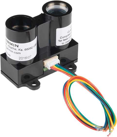
A 1-dimensional (1D) LIDAR sensor works much like an ultrasonic sensor - it measures the distance to the nearest object more or less along a line in front of it. 1D LIDAR sensors can often be more-reliable than ultrasonics, as they have narrower “beam profiles” and are less susceptible to interference. Pictured above is the Garmin LIDAR-Lite Optical Distance Sensor.
1D LIDAR sensors generally output an analog voltage proportional to the measured distance, and thus connect to the roboRIO’s analog input ports or to one of the roboRIO’s serial buses.
2-Dimensional LIDAR
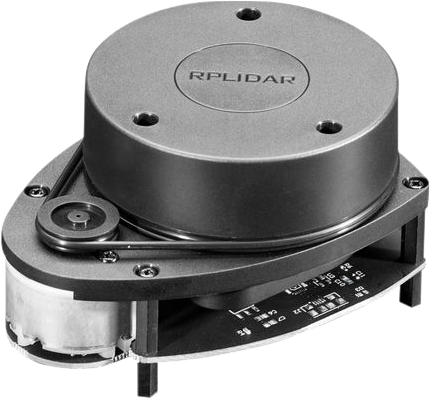
A 2-dimensional (2D) LIDAR sensor measures distance in all directions in a plane. Generally, this is accomplished (more-or-less) by simply placing a 1D LIDAR sensor on a turntable that spins at a constant rate.
Since, by nature, 2D LIDAR sensors need to send a large amount of data back to the roboRIO, they almost always connect to one of the roboRIO’s serial buses.
Caveats
LIDAR sensors do suffer from a few common drawbacks:
Like ultrasonics, LIDAR relies on the reflection of the emitted pulse back to the sensor. Thus, LIDAR critically depends on the reflectivity of the material in the wavelength of the laser. The FRC field wall is made of polycarbonate, which tends to be transparent in the infrared wavelength (which is what is generally legal for FRC use). Thus, LIDAR tends to struggle to detect the field barrier.
2D LIDAR sensors (at the price range legal for FRC use) tend to be quite noisy, and processing their measured data (known as a “point cloud”) can involve a lot of complex software. Additionally, there are very few 2D LIDAR sensors made specifically for FRC, so software support tends to be scarce.
As 2D LIDAR sensors rely on a turntable to work, their update rate is limited by the rate at which the turntable spins. For sensors in the price range legal for FRC, this often means that they do not update their values particularly quickly, which can be a limitation when the robot (or the targets) are moving.
Additionally, as 2D LIDAR sensors are limited in angular resolution, the spatial resolution of the point cloud is worse when targets are further away.
Triangulating Rangefinders
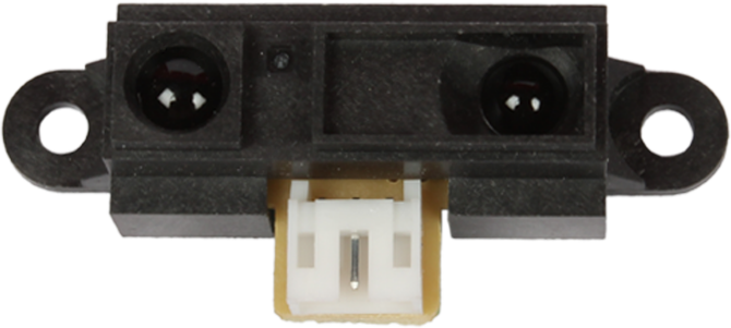
Triangulating rangefinders (often called “IR rangefinders,” as they commonly function in the infrared wavelength band) are another common type of rangefinder used in FRC®. The sensor shown above is a common Sharp-brand sensor
Unlike LIDAR, triangulating rangefinders do not measure the time between the emission of a pulse and the receiving of a reflection. Rather, most IR rangefinders work by emitting a constant beam at a slight angle, and measuring the position of the reflected beam. The closer the point of contact of the reflected beam to the emitter, the closer the object to the sensor.
Using IR rangefinders

IR Rangefinders generally output an analog voltage proportional to the distance to the target, and thus connect to the analog input ports on the RIO.
Caveats
IR rangefinders suffer similar drawbacks to 1D LIDAR sensors - they are very sensitive to the reflectivity of the target in the wavelength of the emitted laser.
Additionally, while IR rangefinders tend to offer better resolution than LIDAR sensors when measuring at short distances, they are also usually more sensitive to differences in orientation of the target, especially if the target is highly-reflective (such as a mirror).
Serial Buses
In addition to the digital and analog inputs, the roboRIO also offers several methods of serial communication with peripheral devices.
Both the digital and analog inputs are highly limited in the amount of data that can be send over them. Serial buses allow users to make use of far more-robust and higher-bandwidth communications protocols with sensors that collect large amounts of data, such as inertial measurement units (IMUs) or 2D LIDAR sensors.
Types of supported serial buses
The roboRIO supports many basic types of serial communications:
Additionally, the roboRIO supports communications with peripheral devices over the CAN bus. However, as the FRC® CAN protocol is quite idiosyncratic, relatively few peripheral sensors support it (though it is heavily used for motor controllers).
I2C

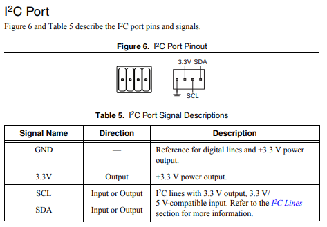
To communicate to peripheral devices over I2C, each pin should be wired to its corresponding pin on the device. I2C allows users to wire a “chain” of slave devices to a single port, so long as those devices have separate IDs set.
The I2C bus can also be used through the MXP expansion port. The I2C bus on the MXP is independent. For example, a device on the main bus can have the same ID as a device on the MXP bus.
SPI

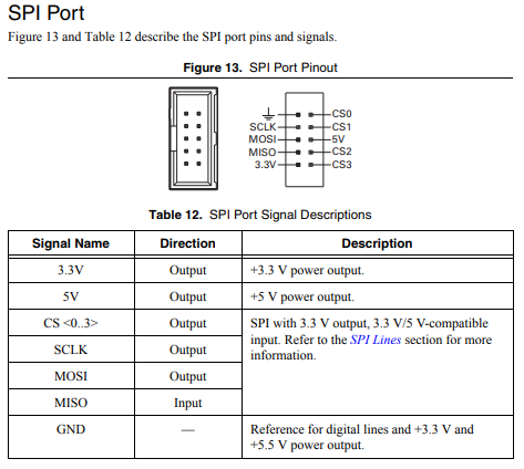
To communicate to peripheral devices over SPI, each pin should be wired to its corresponding pin on the device. The SPI port supports communications to up to four devices (corresponding to the Chip Select (CS) 0-3 pins on the diagram above).
The SPI bus can also be used through the MXP expansion port. The MXP port provides independent clock, and input/output lines and an additional CS.
RS-232

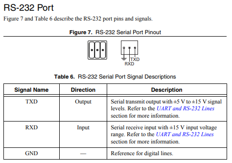
To communicate to peripheral devices over RS-232, each pin should be wired to its corresponding pin on the device.
The RS-232 bus can also be used through the MXP expansion port.
The RoboRIO RS-232 serial port uses RS-232 signaling levels (+/- 15v). The MXP serial port uses CMOS signaling levels (+/- 3.3v).
Note
By default, the onboard RS-232 port is utilized by the roboRIO’s serial console. In order to use it for an external device, the serial console must be disabled using the Imaging Tool or roboRIO Web Dashboard.
USB Client
One of the USB ports on the roboRIO is a USB-B, or USB client port. This can be connected to devices, such as a Driver Station computer, with a standard USB cable.
USB Host

Two of the USB ports on the roboRIO is a USB-A, or USB host port. These can be connected to devices, such as cameras or sensors, with a standard USB cable.
MXP Expansion Port

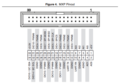
Several of the serial buses are also available for use through the roboRIO’s MXP Expansion Port. This port allows users to make use of many additional digital and analog inputs, as well as the various serial buses.
Many peripheral devices attach directly to the MXP port for convenience, requiring no wiring on the part of the user.
CAN Bus

Additionally, the roboRIO supports communications with peripheral devices over the CAN bus. However, as the FRC CAN protocol is quite idiosyncratic, relatively few peripheral sensors support it (though it is heavily used for motor controllers). One of the advantages of using the CAN bus protocol is that devices can be daisy-chained, as shown below. If power is removed from any device in the chain, data signals will still be able to reach all devices in the chain.
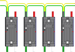
Several sensors primarily use the CAN bus. Some examples include:
CAN Based Time-of-Flight Range/Distance Sensor from playingwithfusion.com
TalonSRX-based sensors, such as the Gadgeteer Pigeon IMU and the SRX MAG Encoder
Power monitoring sensors built into the CTRE Power Distribution Panel (PDP) and the REV Power Distribution Hub (PDH)
More information about using devices connected to the CAN bus can be found in the article about using can devices.
Getting Started with Romi
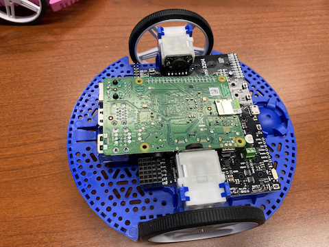
The Romi is a small and inexpensive robot designed for learning about programming FRC robots. All the same tools used for programming full-sized FRC robots can be used to program the Romi. The Romi comes with two drive motors with integrated wheel encoders. It also includes an IMU sensor that can be used for measuring headings and accelerations. Using it is as simple as writing a robot program, and running it on your computer. It will command the Romi to follow the steps in the program.
Romi Hardware & Assembly
To get started with the Romi, you will need to have the necessary hardware.
Romi Kit from Pololu – Order qualifies for free shipping
Raspberry Pi – 3B+ or 4
Micro SD card reader - if you don’t already have one
6 AA batteries – Rechargeable is best (don’t forget the charger)
Assembly
The Romi Robot Kit for FIRST comes pre-soldered and only has to be put together before it can be used. Once you have gathered all the materials you can begin assembly:
Align the motor clips with the chassis as indicated and press them firmly into the chassis until the bottom of the clips are even with the bottom of the chassis (you may hear several clicks).
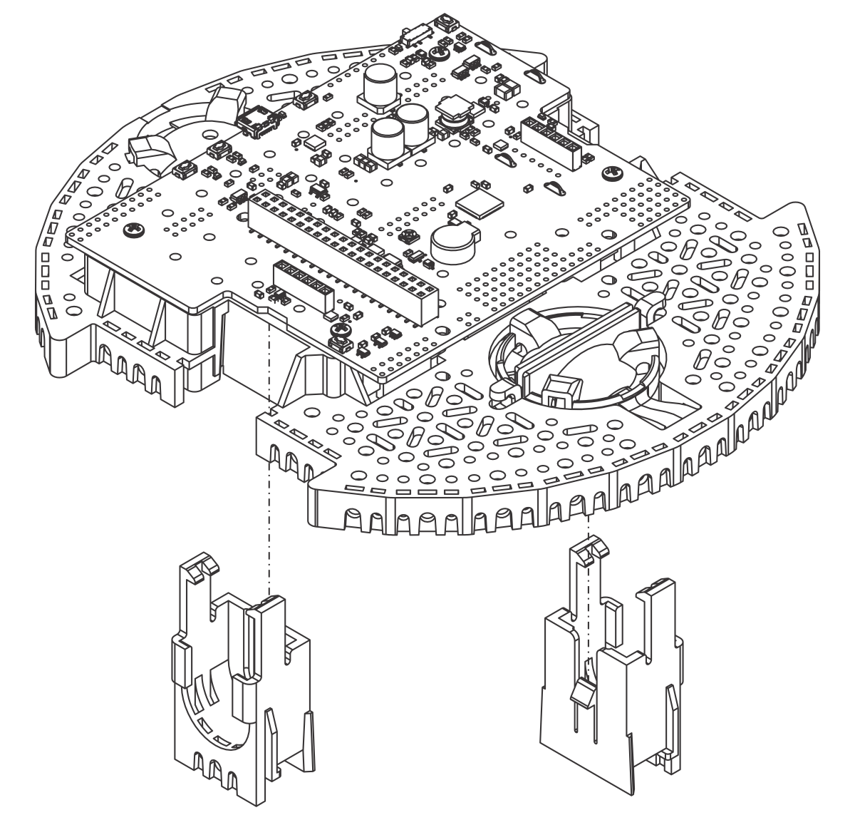
Push the Mini Plastic Gearmotors into the motor clips until they snap into place. Note that the motor blocks the clip release, so if you need to remove a motor bracket later, you will first need to remove the motor. The Mini Plastic Gearmotors that come with the kit have extended motor shafts to enable quadrature encoders for position feedback.
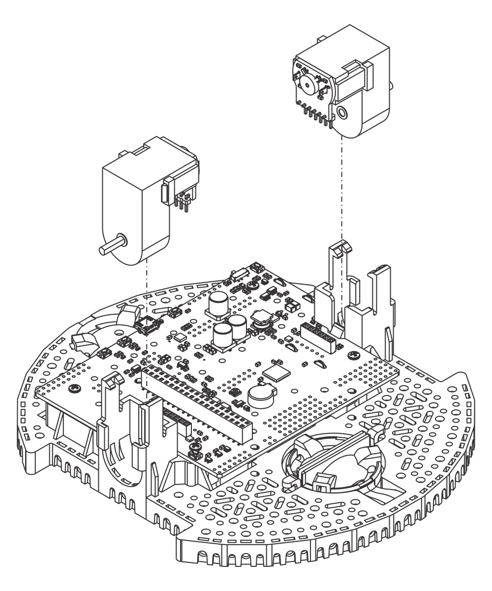
Press the wheels onto the output shafts of the motors until the motor shaft is flush with the outer face of the wheel. One way to do this is to set the wheel on a flat surface and line the chassis up with it so that the flat part of the motor’s D-shaft lines up correctly with the wheel. Then, lower the chassis, pressing the motor shaft into the wheel until it contacts the surface.
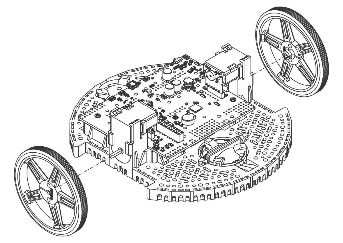
Flip the chassis upside down and place the three rollers for the rear ball caster into the cutouts in the chassis. Place the 1″ plastic ball on top of the three rollers. Then push the ball caster retention clip over the ball and into the chassis so the three legs snap into their respective holes.
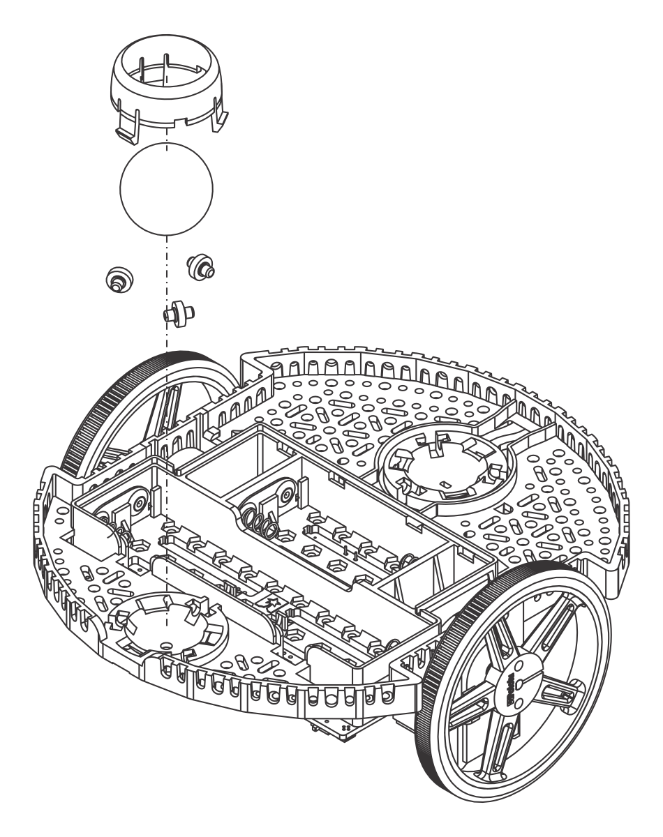
Repeat for the front ball caster so there is a caster on the front and the back of the robot.
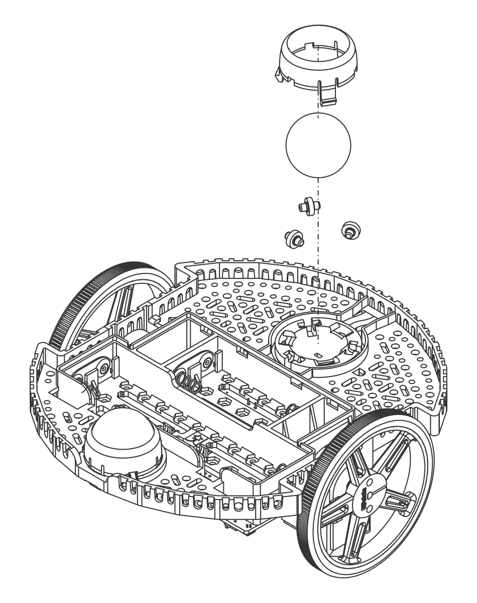
Optional: The front ball caster is supported by a flexible arm that acts as a suspension system. If you want to make it stiffer, you can wrap a rubber band around the two hooks located on either side of the ball caster on the top side of the chassis.
Install the standoffs to support the Raspberry Pi board. Two standoffs (thread side down) mount in the holes on the side of the Romi board closest to the “Romi 32U4” label as shown in the picture. The nuts for these standoffs are inside the battery compartment. The other two standoffs go into the holes on the opposite side of the board. To attach them, you will need a needle-nose pliers to hold the nut while you screw in the standoffs. The circled holes in the image below show where the standoffs should go.
The chassis works with four or six AA batteries (we recommend using rechargeable AA NiMH cells). The correct orientation for the batteries is indicated by the battery-shaped holes in the Romi chassis as well as the + and - indicators in the chassis itself.
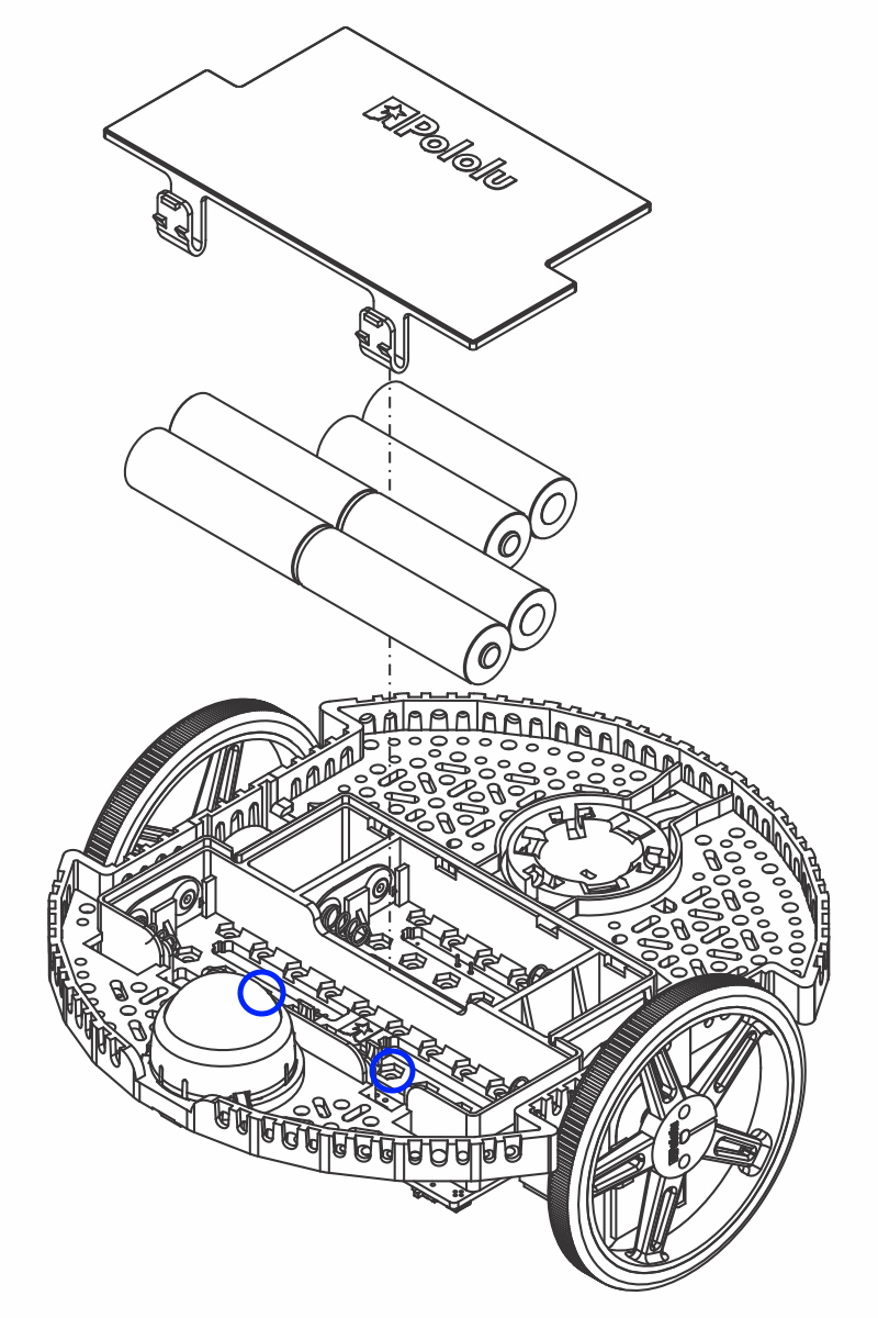
Attach the Raspberry Pi board upside down, carefully aligning the 2x20 pin connector on the Pi with the 2x20 pin socket on the Romi. Push with even pressure taking care to not bend any of the pins. Once inserted, use the supplied screws to fasten the Raspberry Pi board to the standoffs that were installed in a previous step.
Note
Two of the screws will require placing a nut in a hexagonal hole inside the battery compartment. The locations are shown by the blue circles in the image above.
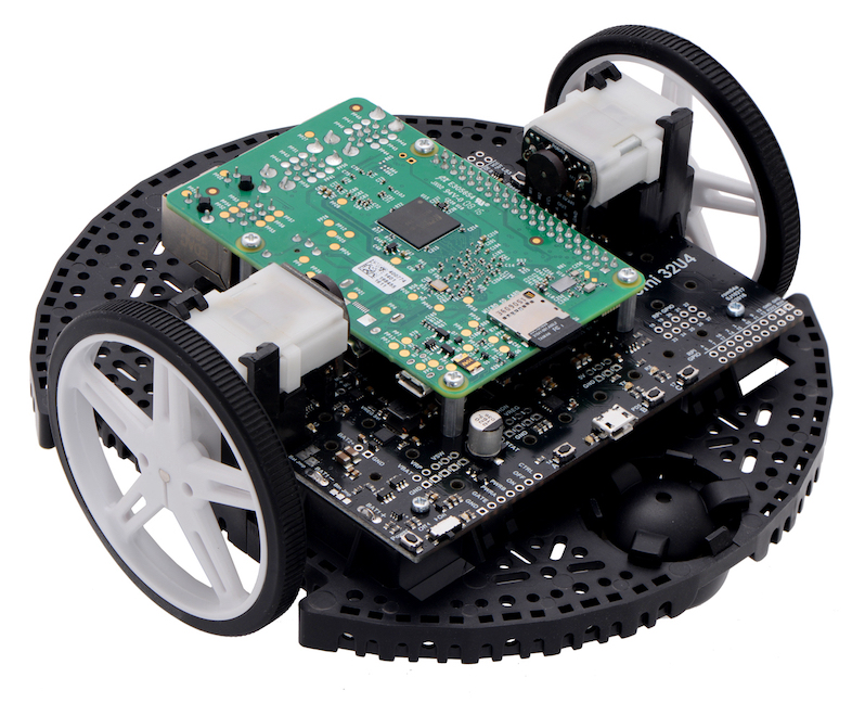
The assembly of your Romi chassis is now complete!
Imaging your Romi
The Romi has 2 microprocessor boards:
A Raspberry Pi that handles high level communication with the robot program running on the desktop and
A Romi 32U4 Control Board that handles low level motor and sensor operation.
Both boards need to have firmware installed so that the robot operate properly.
Raspberry Pi
Download
The Raspberry Pi firmware is based on WPILibPi (formerly FRCVision) and must be downloaded and written to the Raspberry Pi micro SD card. Click on Assets at the bottom of the description to see the available image files:
Be sure to download the Romi version and not the standard release of WPILibPi. The Romi version is suffixed with -Romi. See the below image for an example.
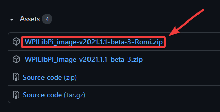
Imaging
The procedure for installing the image is described here: WPILibPi Installation.
Wireless Network Setup
Perform the following steps to get your Raspberry Pi ready to use with the Romi:
Turn the Romi on by sliding the power switch on the Romi 32U4 board to the on position. The first time it is started with a new image it will take approximately 2-3 minutes to boot while it resizes the file system and reboots. Subsequent times it will boot in less than a minute.
Using your computer, connect to the Romi WiFi network using the SSID
WPILibPi-<number>(where<number>is based on the Raspberry Pi serial number) with the WPA2 passphraseWPILib2021!.
Note
If powering on the Raspberry Pi in an environment with multiple WPILibPi-running Raspberry Pis, the SSID for a particular Raspberry Pi is also announced audibly through the headphone port. The default SSID is also written to the /boot/default-ssid.txt file, which can be read by inserting the SD card (via a reader) into a computer and opening the boot partition.
Open a web browser and connect to the Raspberry Pi dashboard at either
http://10.0.0.2/orhttp://wpilibpi.local/.
Note
The image boots up read-only by default, so it is necessary to click the Writable button to make changes. Once done making changes, click the Read-Only button to prevent memory corruption.
Select Writable at the top of the dashboard web page.
Change the default password for your Romi by setting a new password in the
WPA2 Passphrasefield.Press the Save button at the bottom of the page to save changes.
Change the network SSID to a unique name if you plan on operating your Romi on wireless network with other Romis.
Reconnect to the Romi’s WiFi network with the new password you set.
Be sure to set the Dashboard to Read-only when all the changes have been completed.
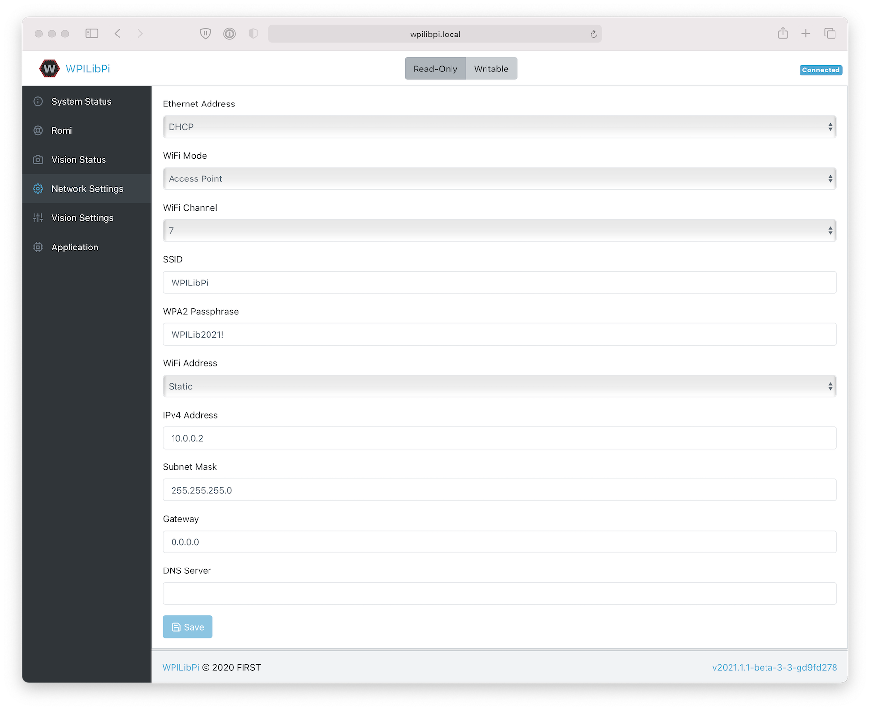
32U4 Control Board
The Raspberry Pi can now be used to write the firmware image to the 32U4 Control Board.
Turn off the Romi
Connect a USB A to micro-B cable from one of the Raspberry Pi’s USB ports to the micro USB port on the 32U4 Control Board.
Turn on the Romi and connect to its Wifi network and connect to the web dashboard as in the previous steps.
On the
Romiconfiguration page, press the Update Firmware button.
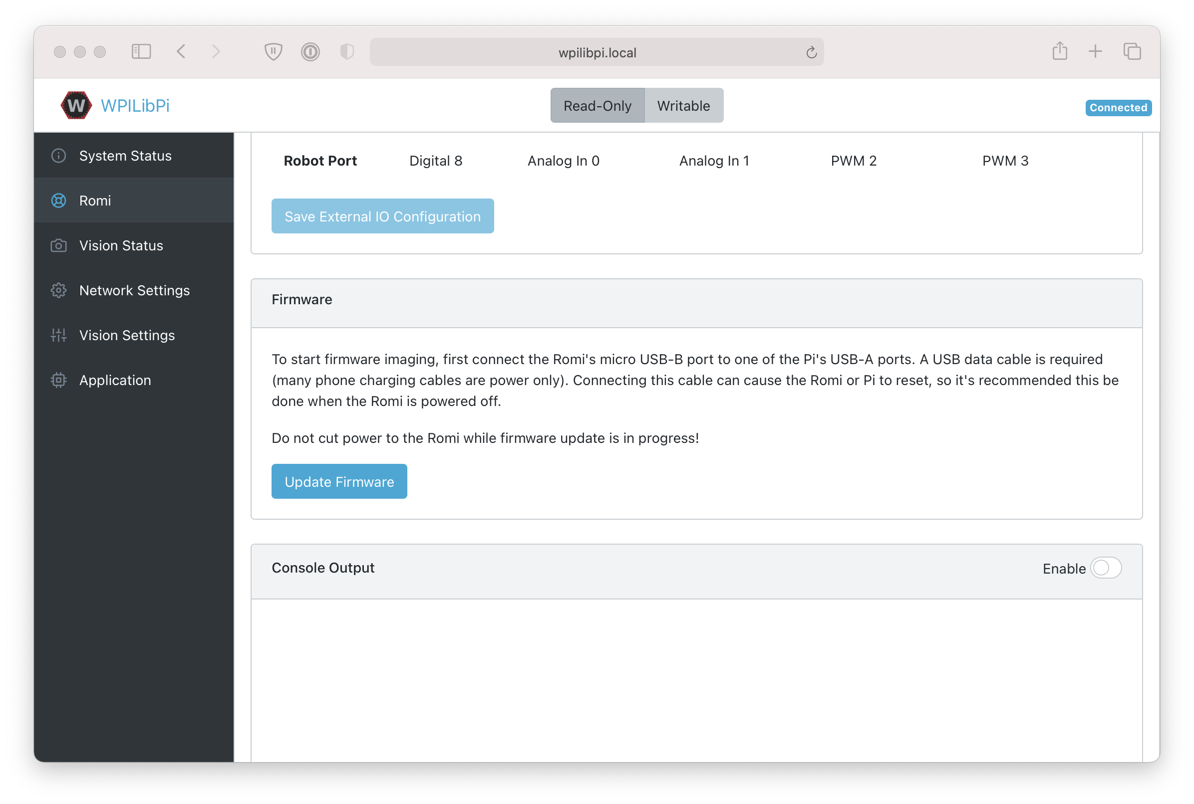
A console will appear showing a log of the firmware deploy process. Once the firmware has been deployed to the 32U4 Control Board, the message avrdude done. Thank you. will appear.
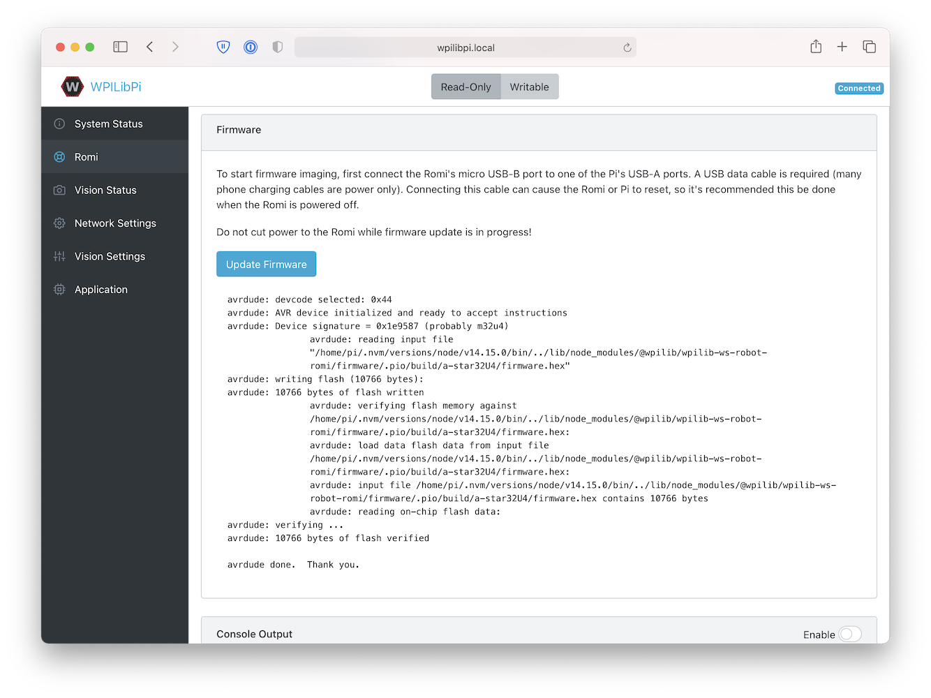
Getting to know your Romi
Directional Conventions
The front of the Romi is where the Raspberry Pi USB ports, GPIO pins and suspended caster wheel are.
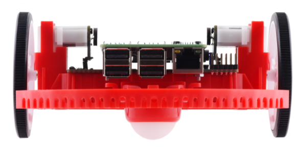
In all Romi documentation, references to driving forward use the above definition of “front”.
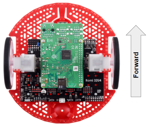
Hardware, Sensors and GPIO
The Romi has the following built-in hardware/peripherals:
2x geared motors with encoders
1x Inertial Measurement Unit (IMU)
3x LEDs (green, yellow, red)
3x pushbuttons (marked A, B, and C)
5x configurable GPIO channels (EXT)
Buzzer
Note
The Buzzer is currently not supported by WPILib.
Motors, Wheels and Encoders
The motors used on the Romi have a 120:1 gear reduction, and a no-load output speed of 150 RPM at 4.5V. The free current is 0.13 amps and the stall current is 1.25 amps. Stall torque is 25 oz-in (0.1765 N-m) but the built-in safety clutch might start slipping at lower torques.
The wheels have a diameter of 70mm (2.75”). They have a trackwidth of 141mm (5.55”).
The encoders are connected directly to the motor output shaft and have 12 Counts Per Revolution (CPR). With the provided gear ratio, this nets 1440 counts per wheel revolution.
The motor PWM channels are listed in the table below.
Channel |
Romi Hardware Component |
|---|---|
PWM 0 |
Left Motor |
PWM 1 |
Right Motor |
Note
The right motor will spin in a backward direction when positive output is applied. Thus, the corresponding motor controller needs to be inverted in robot code.
The encoder channels are listed in the table below.
Channel |
Romi Hardware Component |
|---|---|
DIO 4 |
Left Encoder Quadrature Channel A |
DIO 5 |
Left Encoder Quadrature Channel B |
DIO 6 |
Right Encoder Quadrature Channel A |
DIO 7 |
Right Encoder Quadrature Channel B |
Note
By default, the encoders count up when the Romi moves forward.
Inertial Measurement Unit
The Romi includes an STMicroelectronics LSM6DS33 Inertial Measurement Unit (IMU) which contains a 3-axis gyro and a 3-axis accelerometer.
The accelerometer has selectable sensitivity of 2G, 4G, 8G, and 16G. The gyro has selectable sensitivity of 125 Degrees Per Second (DPS), 250 DPS, 500 DPS, 1000 DPS and 2000 DPS.
The Romi Web UI also provides a means to calibrate the gyro and measure its zero-offsets before use with robot code.
Onboard LEDs and Push Buttons
The Romi 32U4 control board has 3 push buttons and 3 LEDs onboard that are exposed as Digital IO (DIO) channels to robot code.
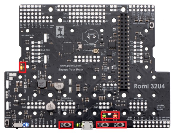
DIO Channel |
Romi Hardware Component |
|---|---|
DIO 0 |
Button A (input only) |
DIO 1 |
Button B (input), Green LED (output) |
DIO 2 |
Button C (input), Red LED (output) |
DIO 3 |
Yellow LED (output only) |
Writes to DIO 0, 4, 5, 6 and 7 will result in no-ops.
Configurable GPIO Pins
The control board has 5 configurable GPIO pins (named EXT0 through EXT4) that allow a user to connect external sensors and actuators to the Romi.
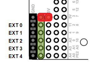
All 5 pins support the following modes: Digital IO, Analog In, PWM (with the exception of EXT 0, which only supports Digital IO and PWM). The mode of the ports can be configured with The Romi Web UI.
The GPIO channels are exposed via a 3-pin, servo style interface, with connections for Ground, Power and Signal (with the Ground connection being closest to the edge of the board, and the signal being closest to the inside of the board).
The power connections for the GPIO pins are initially left unconnected, but can be hooked into the Romi’s on-board 5V supply by using a jumper to connect the 5V pin to the power bus (as seen in the image above). Additionally, if more power than the Romi can provide is needed, the user can provide their own 5V power supply and connect it directly to power bus and ground pins.
GPIO Default Configuration
The table below shows the default configuration of the GPIO pins (EXT0 through EXT4). The Romi Web UI allows the user to customize the functions of the 5 configurable GPIO pins. The UI will also provide the appropriate WPILib channel/device mappings on screen once the IO configuration is complete.
Channel |
Ext Pin |
|---|---|
DIO 8 |
EXT0 |
Analog In 0 |
EXT1 |
Analog In 1 |
EXT2 |
PWM 2 |
EXT3 |
PWM 3 |
EXT4 |
Romi Hardware Support
The Romi robot, having a different hardware architecture than a roboRIO, is compatible with a subset of commonly used FRC control system components.
Compatible Hardware
In general, the Romi is compatible with the following:
Simple Digital Input/Output devices (e.g. bumper switches, single LEDs)
Standard RC-style PWM output devices (e.g. servos, PWM based motor controllers)
Analog Input sensors (e.g distance sensors that report distance as a voltage)
Incompatible Hardware
Due to hardware limitations, the Romi Robot is not compatible with the following:
Encoders other than the Romi-integrated encoders
“Ping” style ultrasonic sensors (which require 2 DIO channels)
Timing based sensors
CAN based devices
Romi built-in buzzer
Compatible Classes
All classes listed here are supported by the Romi Robot. If a class is not listed here, assume that it is not supported and will not work.
PWM Motor Controllers (i.e.
Spark)EncoderAnalogInputDigitalInputDigitalOutputServoBuiltInAccelerometer
The following classes are provided by the Romi Vendordep.
RomiGyroRomiMotorOnboardIO
The Romi Web UI
The Romi Web UI comes installed as part of the WPILibPi Raspberry Pi image. It is accessible by clicking on the Romi tab in the navigation bar of the main WPILibPi Web UI.
The rest of this section will walk through the various parts of the Romi Web UI and describe the relevant functionality.
Background Service Status
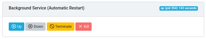
This section of the Romi Web UI provides information about the currently running Romi Web Service (which is what allows WPILib to talk to the Romi). The UI provides controls to bring the service up/down as well as shows the current uptime of the web service.
Note
Users will not need to use the functionality in this section often, but it can be useful for troubleshooting.
Romi Status
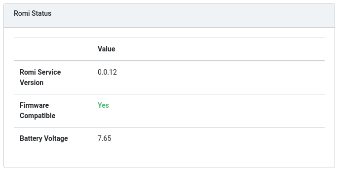
This section provides information about the Romi, including the service version, battery voltage, and whether or not the currently installed firmware on the Romi 32U4 board is compatible with the current version of the web service.
Note
If the firmware is not compatible, see the section on Imaging your Romi
Web Service Update
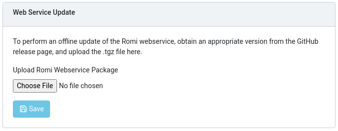
Note
The Raspberry Pi must be in Writable mode for this section to work.
The Romi WPILibPi image ships with the latest (at publication time) version of the Romi web service. To support upgrading to newer versions of the Romi web service, this section allows users to upload a pre-built bundle that can be obtained via the Romi web service GitHub releases page.
To perform an upgrade, download the appropriate .tgz file from the GitHub Releases page. Next, select the downloaded .tgz file and click Save. The updated web service bundle will be uploaded to the Raspberry Pi, and be installed. After a short moment, the Romi Status section should update itself with the latest version information.
External IO Configuration
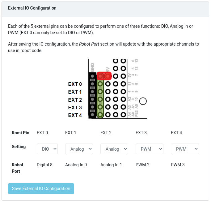
This section allows users to configure the 5 external GPIO channels on the Romi.
Note
The Raspberry Pi must be in Writable mode for this section to work.
To change the configuration of a GPIO channel, select an appropriate option from the dropdown lists. All channels (with the exception of EXT 0) support Digital IO, Analog In and PWM as channel types. Once the appropriate selections are made, click on Save External IO Configuration. The web service will then restart and pick up the new IO configuration.
The “Robot Port” row provides the appropriate WPILib mapping for each configured GPIO channel. For example, EXT 0 is configured as a Digital IO channel, and will be accessible in WPILib as a DigitalInput (or DigitalOutput) channel 8.
IMU Calibration
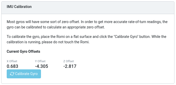
Note
The Raspberry Pi must be in Writable mode for this section to work.
This section allows users to calibrate the gyro on the Romi. Gyros usually have some sort of zero-offset error, and calibration allows the Romi to calculate the offset and use it in calculations.
To begin calibration, place the Romi on a flat, stable surface. Then, click the Calibrate Gyro button. A progress bar will appear, showing the current calibration process. Once calibration is complete, the latest offset values will be displayed on screen and registered with the Romi web service.
These offset values are saved to disk and persist between reboots.
Firmware
Note
See the section on Imaging your Romi
Console Output
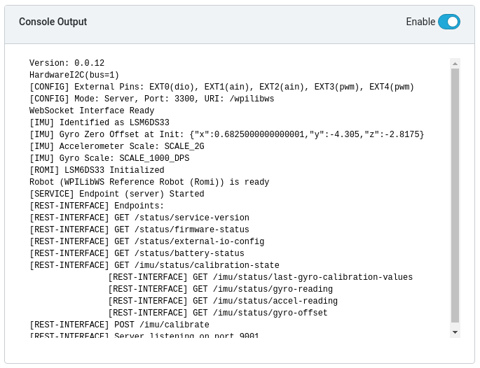
When enabled, this section allows users to view the raw console output that the Romi web service provides. This is useful for troubleshooting issues with the Romi, or just to find out more about what goes on behind the scenes.
Bridge Mode
Bridge mode allows your Romi robot to connect to a WiFi network instead of acting as an Access Point (AP). This is especially useful in remote learning environments, as you can use the internet while using the Romi without extra hardware.
Note
Bridge mode is not likely to work properly in restricted network environments (Educational Institutions).
Enable Writable in the top menu.
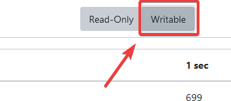
Click on Network Settings.
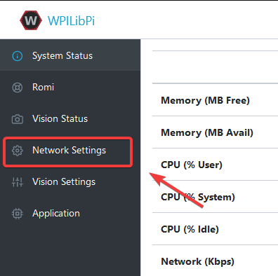
The following network settings must be applied:
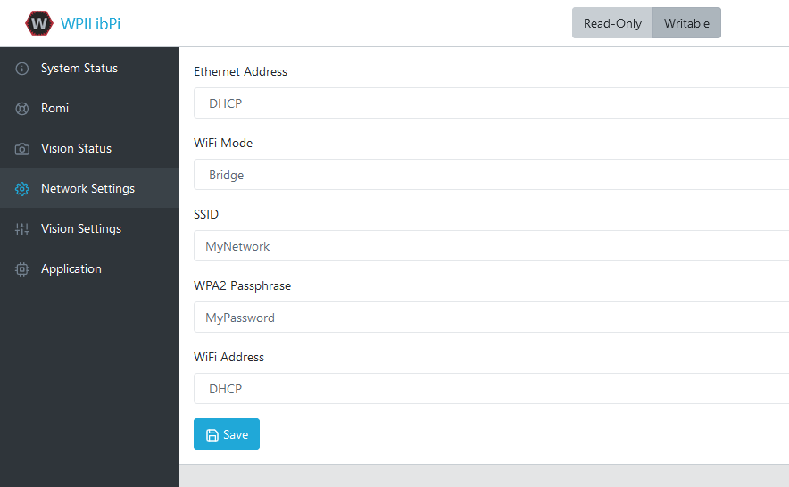
Ethernet: DHCP
WiFi Mode: Bridge
SSID: SSID (name) of your network
WPA2 Passphrase: Password of your wifi network
WiFi Address: DHCP
Once the settings are applied, please reboot the Romi. You should now be able to navigate to wpilibpi.local in your web browser while connected to your specified network.
Unable to Access Romi
If the Romi has the correct bridge settings and you are unable to access it, we have a few workarounds.
Ethernet into the Romi
Reimage the Romi
Some restricted networks can interfere with the hostname of the Romi resolving, you can workaround this by using Angry IP Scanner to find the IP address.
Warning
Angry IP Scanner is flagged by some antivirus as spyware as it pings devices on your network! It is a safe application!
Programming the Romi
Writing a program for the Romi is very similar to writing a program for a regular FRC robot. In fact, all the same tools (Visual Studio Code, Driver Station, SmartDashboard, etc) can be used with the Romi.
Creating a Romi Program
Creating a new program for a Romi is like creating a normal FRC program, similar to the Zero To Robot programming steps.
WPILib comes with two templates for Romi projects, including one based on TimedRobot, and a Command-Based project template. Additionally, an example project is provided which showcases some of the built-in functionality of the Romi. This article will walk through creating a project from this example.
Note
In order to program the Romi using C++, a compatible C++ desktop compiler must be installed. See Robot Simulation - Additional C++ Dependency.
Creating a New WPILib Romi Project
Bring up the Visual Studio Code command palette with Ctrl+Shift+P, and type “New project” into the prompt. Select the “Create a new project” command:
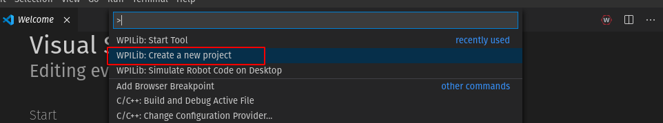
This will bring up the “New Project Creator Window”. From here, click on “Select a project type (Example or Template), and pick “Example” from the prompt that appears:
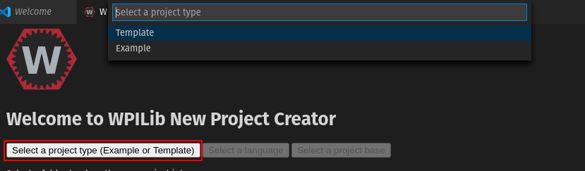
Next, a list of examples will appear. Scroll through the list to find the “RomiReference” example:
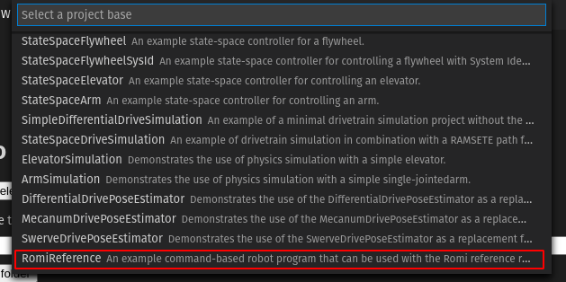
Fill out the rest of the fields in the “New Project Creator” and click “Generate Project” to create the new robot project.
Running a Romi Program
Once the robot project is generated, it is essentially ready to run. The project has a pre-built Drivetrain class and associated default command that lets you drive the Romi around using a joystick.
One aspect where a Romi project differs from a regular FRC robot project is that the code is not deployed directly to the Romi. Instead, a Romi project runs on your development computer and leverages the WPILib simulation framework to communicate with the Romi robot.
To run a Romi program, first, ensure that your Romi is powered on. Next, connect to the WPILibPi-<number> WiFi network broadcast by the Romi. If you changed the Romi network settings (for example, to connect it to your own WiFi network) you may change the IP address that your program uses to connect to the Romi. To do this, open the build.gradle file and update the envVar line to the appropriate IP address.
Now to start your Romi robot code, open the WPILib Command Palette (type Ctrl+Shift+P) and select “Simulate Robot Code”, or press F5.
If all goes well, you should see a line in the console output that reads “HALSimWS: WebSocket Connected”:
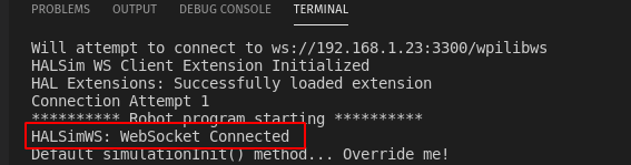
Your Romi code is now running!
Programming the Romi (LabVIEW)
Writing a LabVIEW program for the Romi is very similar to writing a program for a regular roboRIO based robot. In fact, all the same tools can be used with the Romi.
Creating a Romi Project
Creating a new program for a Romi is no different than creating a normal FRC |reg| program, similar to the Zero To Robot programming steps. Initially, you may wish to create a separate project for use on just the Romi as the Romi hardware may be connected to different ports than on your roboRIO robot.
The Romi Robot used PWM ports 0 and 1 for left and right side respectively.
Installing the WebSockets VI
One aspect where a Romi project differs from a regular FRC |reg| robot project is that the code is not deployed directly to the Romi. Instead, a Romi project runs on your development computer, and leverages the WPILib simulation framework to communicate with the Romi robot. WebSockets is the protocol that LabVIEW uses to converse with the Romi.
Open the VI Package Manager application. Type websockets into the search box in the top right. Select the VI by LabVIEW Tools Network.
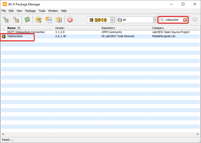
Changing the Project Target
The primary step needed to run your LabVIEW program on the Romi is to change the target to the Desktop. To change the project target, locate the Robot Main VI in the Project Explorer and click and drag it from the Target section to the My Computer section.
Setting the Target IP
By default, your LabVIEW program will attempt to connect to a Romi with the IP address of 10.0.0.2. If you wish to use a different IP, you can specify it as an input to the Driver Station Start Communication VI inside Robot Main. Locate the pink input terminal for Simulation URL then right-click and select Create Constant to create a constant pre-filled with the default value. You can then modify the IP address portion of the text, taking care to leave the protocol section (at the beginning) and port and suffix (at the end) the same.
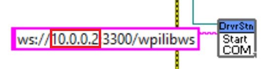
Running a Romi Program
To run a Romi program, first, ensure that your Romi is powered on. Once you connect to the WPILibPi-<number> network broadcast by the Romi, press the white Run arrow to start running the Romi program on your computer.
Your Romi code is now running! The program will automatically attempt to connect to either the IP you have specified, or the default if you have not specified an IP.
It is recommended to run the Driver Station software on the same computer as the LabVIEW code. Once your program successfully connects to the Driver Station, it will automatically notify the Driver Station that the code is running on the Desktop, allowing the Driver Station to connect without you changing any information inside the Driver Station. Next, you’ll need to point the Driver Station to your Romi. This is done by setting the team number to 127.0.0.1. You can then use the controls in the Driver Station to set the robot mode and enable/disable as normal.
Using the Gyro or Encoder
The gyro that is available on the Romi is available using the RomiGyro functions. This is located under
- WPI Robotics Library
- Sensors
- Third Party Libraries
- RomiGyro
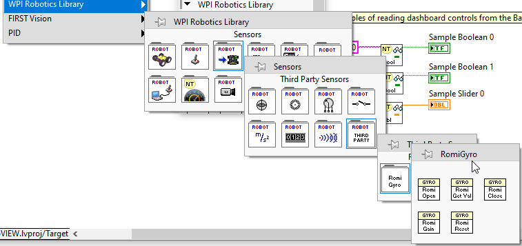
The encoders can be used using the standard encoder function. The DIO ports are:
Left (4, 5)
Right (6, 7)
Networking Introduction
This section outlines basic robot configuration and usage relating to communication between the driver station and roboRIO.
Networking Basics
What is an IP Address?
An IP address is a unique string of numbers, separated by periods that identifies each device on a network. Each IP address is divided up into 4 sections (octets) ranging from 0-255.
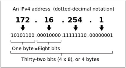
As shown above, this means that each IP address is a 32-bit address meaning there are 232 addresses, or nearly 4,300,000,000 addresses possible. However, most of these are used publicly for things like web servers.
This brings up our first key point of IP Addressing: Each device on the network must have a unique IP address. No two devices can have the same IP address, otherwise collisions will occur.
Since there are only 4-billion addresses, and there are more than 4-billion computers connected to the internet, we need to be as efficient as possible with giving out IP addresses. This brings us to public vs. private addresses.
Public vs Private IP Addresses
To be efficient with using IP Addresses, the idea of “Reserved IP Ranges” was implemented. In short, this means that there are ranges of IP Addresses that will never be assigned to web servers, and will only be used for local networks, such as those in your house.
Key point #2: Unless you a directly connecting to your internet provider’s basic modem (no router function), your device will have an IP Address in one of these ranges. This means that at any local network, such as: your school, work office, home, etc., your device will 99% of the time have an IP address in a range listed below:
Class |
Bits |
Start Address |
End Address |
Number of Addresses |
|---|---|---|---|---|
A |
24 |
10.0.0.0 |
10.255.255.255 |
16,777,216 |
B |
20 |
172.16.0.0 |
172.31.255.255 |
1,048,576 |
C |
16 |
192.168.0.0 |
192.168.255.255 |
65,536 |
These reserved ranges let us assign one “unreserved IP Address” to an entire house, and then use multiple addresses in a reserved range to connect more than one computer to the internet. A process on the home’s internet router known as NAT (Network Address Translation), handles the process of keeping track which private IP is requesting data, using the public IP to request that data from the internet, and then passing the returned data back to the private IP that requested it. This allows us to use the same reserved IP addresses for many local networks, without causing any conflicts. An image of this process is presented below.

Note
For the FRC® networks, we will use the 10.0.0.0 range. This range allows us to use the 10.TE.AM.xx format for IP addresses, whereas using the Class B or C networks would only allow a subset of teams to follow the format. An example of this formatting would be 10.17.50.1 for FRC Team 1750.
How are these addresses assigned?
We’ve covered the basics of what IP addresses are, and which IP addresses we will use for the FRC competition,so now we need to discuss how these addresses will get assigned to the devices on our network. We already stated above that we can’t have two devices on the same network with the same IP Address, so we need a way to be sure that every device receives an address without overlapping. This can be done Dynamically (automatic), or Statically (manual).
Dynamically
Dynamically assigning IP addresses means that we are letting a device on the network manage the IP address assignments. This is done through the Dynamic Host Configuration Protocol (DHCP). DHCP has many components to it, but for the scope of this document, we will think of it as a service that automatically manages the network. Whenever you plug in a new device to the network, the DHCP service sees the new device, then provides it with an available IP address and the other network settings required for the device to communicate. This can mean that there are times we do not know the exact IP address of each device.
What is a DHCP server?
A DHCP server is a device that runs the DHCP service to monitor the network for new devices to configure. In larger businesses, this could be a dedicated computer running the DHCP service and that computer would be the DHCP server. For home networks, FRC networks, and other smaller networks, the DHCP service is usually running on the router; in this case, the router is the DHCP server.
This means that if you ever run into a situation where you need to have a DHCP server assigning IP addresses to your network devices, it’s as simple as finding the closest home router, and plugging it in.
Statically
Statically assigning IP addresses means that we are manually telling each device on the network which IP address we want it to have. This configuration happens through a setting on each device. By disabling DHCP on the network and assigning the addresses manually, we get the benefit of knowing the exact IP address of each device on the network, but because we set each one manually and there is no service keeping track of the used IP addresses, we have to keep track of this ourselves. While statically setting IP addresses, we must be careful not to assign duplicate addresses, and must be sure we are setting the other network settings (such as subnet mask and default gateway) correctly on each device.
What is link-local?
If a device does not have an IP address, then it cannot communicate on a network. This can become an issue if we have a device that is set to dynamically acquire its address from a DHCP server, but there is no DHCP server on the network. An example of this would be when you have a laptop directly connected to a roboRIO and both are set to dynamically acquire an IP address. Neither device is a DHCP server, and since they are the only two devices on the network, they will not be assigned IP addresses automatically.
Link-local addresses give us a standard set of addresses that we can “fall-back” to if a device set to acquire dynamically is not able to acquire an address. If this happens, the device will assign itself an IP address in the 169.254.xx.yy address range; this is a link-local address. In our roboRIO and computer example above, both devices will realize they haven’t been assigned an IP address and assign themselves a link-local address. Once they are both assigned addresses in the 169.254.xx.yy range, they will be in the same network and will be able to communicate, even though they were set to dynamic and a DHCP server did not assign addresses.
IP Addressing for FRC
See the IP Networking Article for more information.
Mixing Dynamic and Static Configurations
While on the field, the team should not notice any issues with having devices set statically in the 10.TE.AM.xx range, and having the field assign DHCP addresses as long as there are no IP address conflicts as referred to in the section above.
In the pits, a team may encounter issues with mixing Static and DHCP devices for the following reason. As mentioned above, DHCP devices will fall back to a link-local address (169.254.xx.yy) if a server isn’t present. For static devices, the IP address will always be the same. If the DHCP server is not present and the roboRIO, driver station, and laptop fall back to link-local addresses, the statically set devices in the 10.TE.AM.xx range will be in a different network and not visible to those with link-local addresses. A visual description of this is provided below:

Warning
When connected via USB to the roboRIO, a Port Forwarding configuration is required to access devices connected to the OpenMesh radio (on the green network shown above).
Available Network Ports
Please see R704 of the 2022 Game Manual for information regarding available network ports.
mDNS
mDNS, or multicast Domain Name System is a protocol that allows us to benefit from the features of DNS, without having a DNS server on the network. To make this clearer, let’s take a step back and talk about what DNS is.
What is DNS?
DNS (Domain Name System) can become a complex topic, but for the scope of this paper, we are going to just look at the high level overview of DNS. In the most basic explanation, DNS is what allows us to relate human-friendly names for network devices to IP Addresses, and keep track of those IP addresses if they change.
Example 1: Let’s look at the site www.google.com. The IP address for this site is 172.217.164.132, however that is not very user friendly to remember!
Whenever a user types www.google.com into their computer, the computer contacts the DNS server (a setting provided by DHCP!) and asks what is the IP address on file for www.google.com. The DNS server returns the IP address and then the computer is able to use that to connect to the Google web site.
Example 2: On your home network, you have a server named MYCOMPUTER that you want to connect to from your laptop. Your network uses DHCP so you don’t know the IP Address of MYCOMPUTER, but DNS allows you to connect just by using the MYCOMPUTER name. Additionally, whenever the DHCP assignments refresh, MYCOMPUTER may end up with a different address, but because you’re connecting by using the MYCOMPUTER name instead of a specific IP address, the DNS record was updated and you’re still able to connect.
This is the second benefit to DNS, and the most relevant for FRC. With DNS, if we reference devices by their friendly name instead of IP Address, we don’t have to change anything in our program if the IP Address changes. DNS will keep track of the changes and return the new address if it ever changes.
DNS for FRC
On the field and in the pits, there is no DNS server that allows us to perform the lookups like we do for the Google web site, but we’d still like to have the benefits of not remembering every IP Address, and not having to guess at every device’s address if DHCP assigns a different address than we expect. This is where mDNS comes into the picture.
mDNS provides us the same benefits as traditional DNS, but is just implemented in a way that does not require a server. Whenever a user asks to connect to a device using a friendly name, mDNS sends out a message asking the device with that name to identify itself. The device with the name then sends a return message including its IP address so all devices on the network can update their information. mDNS is what allows us to refer to our roboRIO as roboRIO-TEAM-FRC.local and have it connect on a DHCP network.
Note
If a device used for FRC does not support mDNS, then it will be assigned an IP Address in the 10.TE.AM.20 - 10.TE.AM.255 range, but we won’t know the exact address to connect and we won’t be able to use the friendly name like before. In this case, the device would need to have a static IP Address.
mDNS - Principles
Multicast Domain Name System (mDNS) is a system which allows for resolution of host names to IP addresses on small networks with no dedicated name server. To resolve a host name a device sends out a multicast message to the network querying for the device. The device then responds with a multicast message containing it’s IP. Devices on the network can store this information in a cache so subsequent requests for this address can be resolved from the cache without repeating the network query.
mDNS - Providers
To use mDNS, an mDNS implementation is required to be installed on your PC. Here are some common mDNS implementations for each major platform:
Windows:
NI mDNS Responder: Installed with the NI FRC Game Tools
Apple Bonjour: Installed with iTunes
OSX:
Apple Bonjour: Installed by default
Linux:
nss-mDNS/Avahi/Zeroconf: Installed and enabled by default on some Linux variants (such as Ubuntu or Mint). May need to be installed or enabled on others (such as Arch)
mDNS - Firewalls
Note
Depending on your PC configuration, no changes may be required, this section is provided to assist with troubleshooting.
To work properly mDNS must be allowed to pass through your firewall. Because the network traffic comes from the mDNS implementation and not directly from the Driver Station or IDE, allowing those applications through may not be sufficient. There are two main ways to resolve mDNS firewall issues:
Add an application/service exception for the mDNS implementation (NI mDNS Responder is
C:\Program Files\National Instruments\Shared\mDNS Responder\nimdnsResponder.exe)Add a port exception for traffic to/from UDP 5353. IP Ranges:
10.0.0.0 - 10.255.255.255172.16.0.0 - 172.31.255.255192.168.0.0 - 192.168.255.255169.254.0.0 - 169.254.255.255224.0.0.251
mDNS - Browser support
Most web-browsers should be able to utilize the mDNS address to access the roboRIO web server as long as an mDNS provider is installed. These browsers include Microsoft Edge, Firefox, and Google Chrome.
USB
If using the USB interface, no network setup is required (you do need the Installing the FRC Game Tools installed to provide the roboRIO USB Driver). The roboRIO driver will automatically configure the IP address of the host (your computer) and roboRIO and the software listed above should be able to locate and utilize your roboRIO.
Ethernet/Wireless
The Programming your Radio will enable the DHCP server on the OpenMesh radio in the home use case (AP mode), if you are putting the OpenMesh in bridge mode and using a router, you can enable DHCP addressing on the router. The bridge is set to the same team based IP address as before (10.TE.AM.1) and will hand out DHCP address from 10.TE.AM.20 to 10.TE.AM.199. When connected to the field, FMS will also hand out addresses in the same IP range.
Summary
IP Addresses are what allow us to communicate with devices on a network. For FRC, these addresses are going to be in the 10.TE.AM.xx range if we are connected to a DHCP server or if they are assigned statically, or in the link-local 169.254.xx.yy range if the devices are set to DHCP, but there is no server present. For more information on how IP Addresses work, see this article by Microsoft.
If all devices on the network support mDNS, then all devices can be set to DHCP and referred to using their friendly names (ex. roboRIO-TEAM-FRC.local). If some devices do not support mDNS, they will need to be set to use static addresses.
If all devices are set to use DHCP or Static IP assignments (with correct static settings), the communication should work in both the pit and on the field without any changes needed. If there are a mix of some Static and some DHCP devices, then the Static devices will connect on the field, but will not connect in the pit. This can be resolved by either setting all devices to static settings, or leaving the current settings and providing a DHCP server in the pit.
IP Configurations
Note
This document describes the IP configuration used at events, both on the fields and in the pits, potential issues and workaround configurations.
TE.AM IP Notation
The notation TE.AM is used as part of IPs in numerous places in this document. This notation refers to splitting your four digit team number into two digit pairs for the IP address octets.
Example: 10.TE.AM.2
Team 12 - 10.0.12.2
Team 122 - 10.1.22.2
Team 1212 - 10.12.12.2
Team 3456 - 10.34.56.2
On the Field
This section describes networking when connected to the Field Network for match play
On the Field DHCP Configuration
The Field Network runs a DHCP server with pools for each team that will hand out addresses in the range of 10.TE.AM.20 to 10.TE.AM.199 with a subnet mask of 255.255.255.0, and a default gateway of 10.TE.AM.4.
When configured for an event, the Team Radio runs a DHCP server with a pool for devices onboard the robot that will hand out addresses in the range of 10.TE.AM.200 to 10.TE.AM.219 with a subnet mask of 255.255.255.0, and a gateway of 10.TE.AM.1.
OpenMesh OM5P-AN or OM5P-AC radio - Static
10.TE.AM.1programmed by KioskroboRIO - DHCP
10.TE.AM.2assigned by the Robot RadioDriver Station - DHCP (“Obtain an IP address automatically”) 10.TE.AM.X assigned by field
IP camera (if used) - DHCP
10.TE.AM.Yassigned by Robot RadioOther devices (if used) - DHCP
10.TE.AM.Zassigned by Robot Radio
On the Field Static Configuration
It is also possible to configure static IPs on your devices to accommodate devices or software which do not support mDNS. When doing so you want to make sure to avoid addresses that will be in use when the robot is on the field network. These addresses are 10.TE.AM.1 for the OpenMesh radio, 10.TE.AM.4 for the field router, and anything greater than 10.TE.AM.20 which may be assigned to a device configured for DHCP or else reserved. The roboRIO network configuration can be set from the webdashboard.
OpenMesh radio - Static
10.TE.AM.1programmed by KioskroboRIO - Static
10.TE.AM.2would be a reasonable choice, subnet mask of255.255.255.0(default)Driver Station - Static
10.TE.AM.5would be a reasonable choice, subnet mask must be255.0.0.0to enable the DS to reach both the robot and FMS Server, without additionally configuring the default gateway. If a static address is assigned and the subnet mask is set to255.255.255.0, then the default gateway must be configured to10.TE.AM.4.IP Camera (if used) - Static
10.TE.AM.11would be a reasonable choice, subnet255.255.255.0should be fineOther devices - Static
10.TE.AM.6-.10or.12-.19(.11 if camera not present) subnet255.255.255.0
In the Pits
Note
New for 2018: There is now a DHCP server running on the wired side of the Robot Radio in the event configuration.
In the Pits DHCP Configuration
OpenMesh radio - Static
10.TE.AM.1programmed by Kiosk.roboRIO -
10.TE.AM.2, assigned by Robot RadioDriver Station - DHCP (“Obtain an IP address automatically”),
10.TE.AM.X, assigned by Robot RadioIP camera (if used) - DHCP,
10.TE.AM.Y, assigned by Robot RadioOther devices (if used) - DHCP,
10.TE.AM.Z, assigned by Robot Radio
In the Pits Static Configuration
It is also possible to configure static IPs on your devices to accommodate devices or software which do not support mDNS. When doing so you want to make sure to avoid addresses that will be in use when the robot is on the field network. These addresses are 10.TE.AM.1 for the OpenMesh radio and 10.TE.AM.4 for the field router.
roboRIO Network Troubleshooting
The roboRIO and FRC® tools use dynamic IP addresses (DHCP) for network connectivity. This article describes steps for troubleshooting networking connectivity between your PC and your roboRIO
Ping the roboRIO using mDNS
The first step to identifying roboRIO networking issues is to isolate if it is an application issue or a general network issue. To do this, click Start -> type cmd -> press Enter to open the command prompt. Type ping roboRIO-####-FRC.local where #### is your team number (with no leading zeroes) and press enter. If the ping succeeds, the issue is likely with the specific application, verify your team number configuration in the application, and check your firewall configuration.
Ping the roboRIO IP Address
If there is no response, try pinging 10.TE.AM.2 (TE.AM IP Notation) using the command prompt as described above. If this works, you have an issue resolving the mDNS address on your PC. The two most common causes are not having an mDNS resolver installed on the system and a DNS server on the network that is trying to resolve the .local address using regular DNS.
Verify that you have an mDNS resolver installed on your system. On Windows, this is typically fulfilled by the NI FRC Game Tools. For more information on mDNS resolvers, see the Network Basics article.
Disconnect your computer from any other networks and make sure you have the OM5P-AN configured as an access point, using the FRC Radio Configuration Utility. Removing any other routers from the system will help verify that there is not a DNS server causing the issue.
Ping Fails
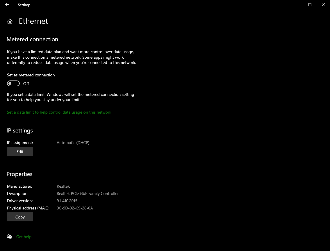
If pinging the IP address directly fails, you may have an issue with the network configuration of the PC. The PC should be configured to Automatic. To check this, click Start -> Settings -> Network & Internet. Depending on your network, select Wifi or Ethernet. Then click on your connected network. Scroll down to IP settings and click Edit and ensure the Automatic (DHCP) option is selected.
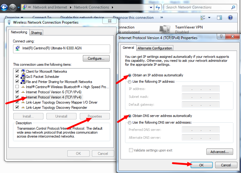
If pinging the IP address directly fails, you may have an issue with the network configuration of the PC. The PC should be configured to Obtain an Address Automatically (also known as DHCP). To check this, click Start -> Control Panel -> Network Connections -> Change adapter settings, then right click on the appropriate interface (usually Local Area Connection for Ethernet or Wireless Network Connection for wireless) and select Properties. Click Internet Protocol Version 4, then click Properties. Make sure both radio buttons are set to Obtain automatically.
USB Connection Troubleshooting
If you are attempting to troubleshoot the USB connection, try pinging the roboRIO’s IP address. As long as there is only one roboRIO connected to the PC, it should be configured as 172.22.11.2. If this ping fails, make sure you have the roboRIO connected and powered, and that you have installed the NI FRC Game Tools. The game tools installs the roboRIO drivers needed for the USB connection.
If this ping succeeds, but the .local ping fails, it is likely that either the roboRIO hostname is configured incorrectly, or you are connected to a DNS server which is attempting to resolve the .local address.
Verify that your roboRIO has been imaged for your team number. This sets the hostname used by mDNS.
Ethernet Connection
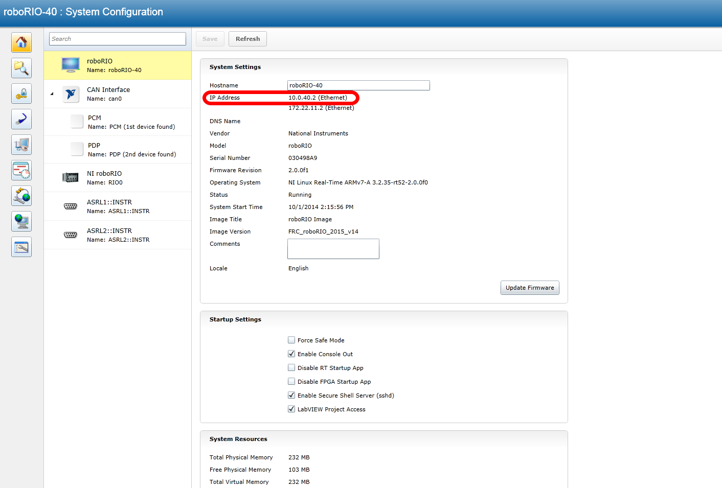
If you are troubleshooting an Ethernet connection, it may be helpful to first make sure that you can connect to the roboRIO using the USB connection. Using the USB connection, open the roboRIO webdashboard and verify that the roboRIO has an IP address on the ethernet interface. If you are tethering to the roboRIO directly this should be a self-assigned 169.*.*.* address, if you are connected to the OM5P-AN radio, it should be an address of the form 10.TE.AM.XX where TEAM is your four digit FRC team number. If the only IP address here is the USB address, verify the physical roboRIO ethernet connection.
Disabling Network Adapters
This is not always the same as turning the adapters off with a physical button or putting the PC into airplane mode. The following steps provide more detail on how to disable adapters.
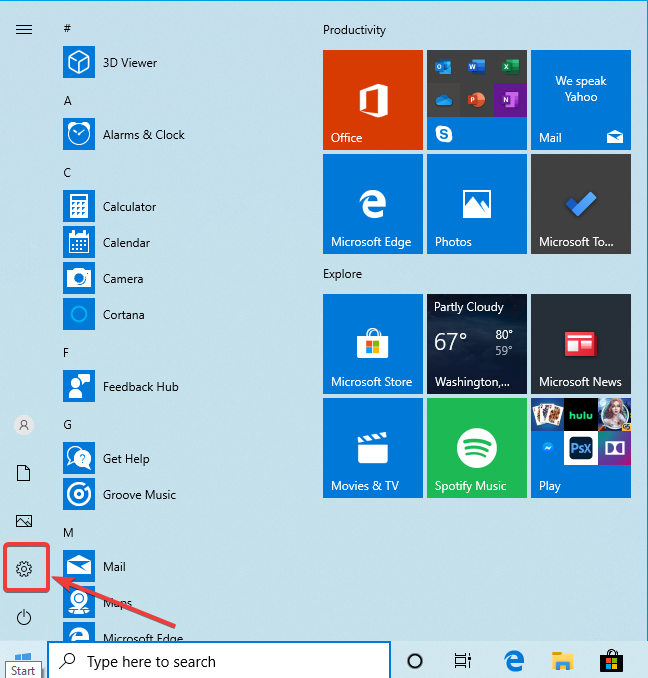
Open the Settings application by clicking on the settings icon.
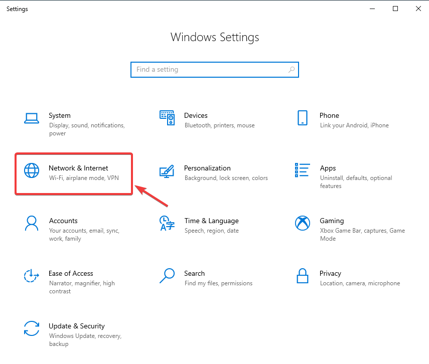
Choose the Network & Internet category.
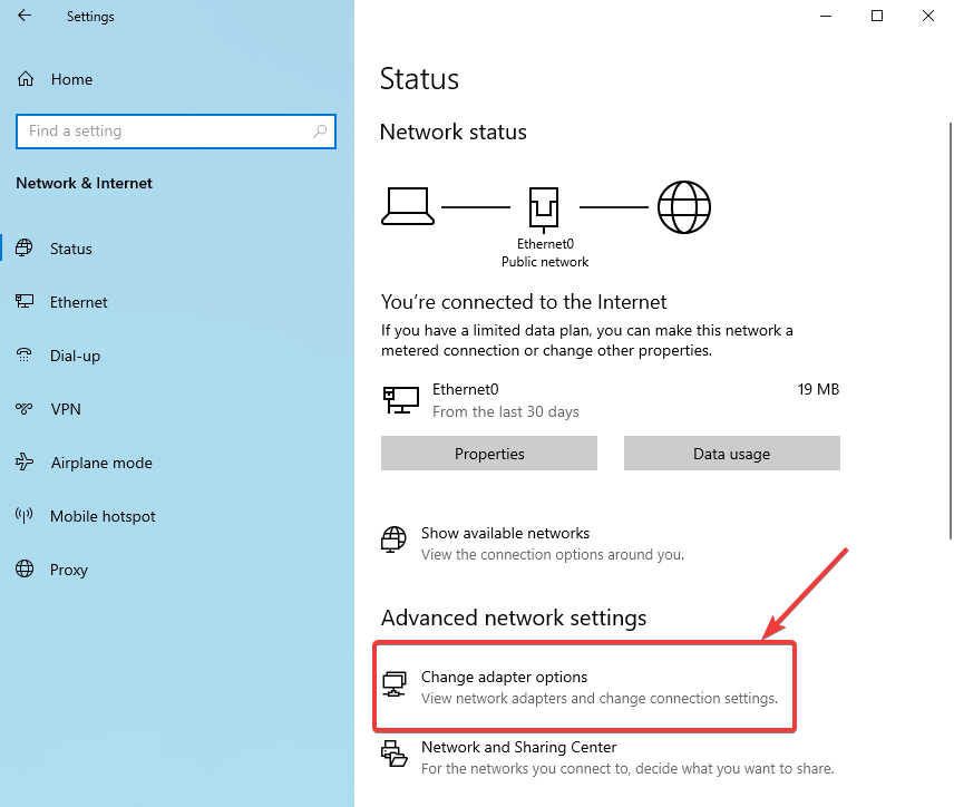
Click on Change adapter options.
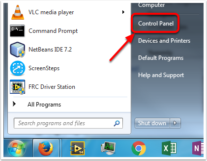
Open the Control Panel by going to Start -> Control Panel
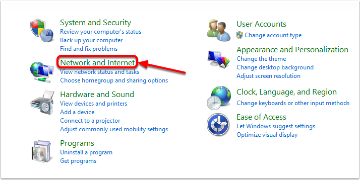
Choose the Network and Internet category.
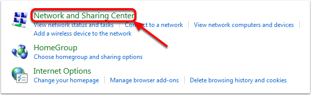
Click Network and Sharing Center
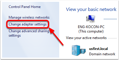
On the left pane, click Change Adapter Settings.
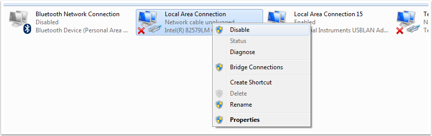
For each adapter other than the one connected to the radio, right click on the adapter and select Disable from the menu.
Proxies
Proxies. Having a proxy enabled may cause issues with the roboRIO networking.
Windows Firewall Configuration
Many of the programming tools used in FRC® need network access for various reasons. Depending on the exact configuration, the Windows Firewall may potentially interfere with this access for one or more of these programs.
Disabling Windows Firewall
Important
Disabling your firewall requires administrator privileges to the PC. Additionally note that disabling the firewall is not recommended for computers that connect to the internet.
The easiest solution is to disable the Windows Firewall. Teams should beware that this does make the PC potentially more vulnerable to malware attacks if connecting to the internet.
Click Start -> Settings
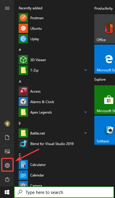
Click Update & Security
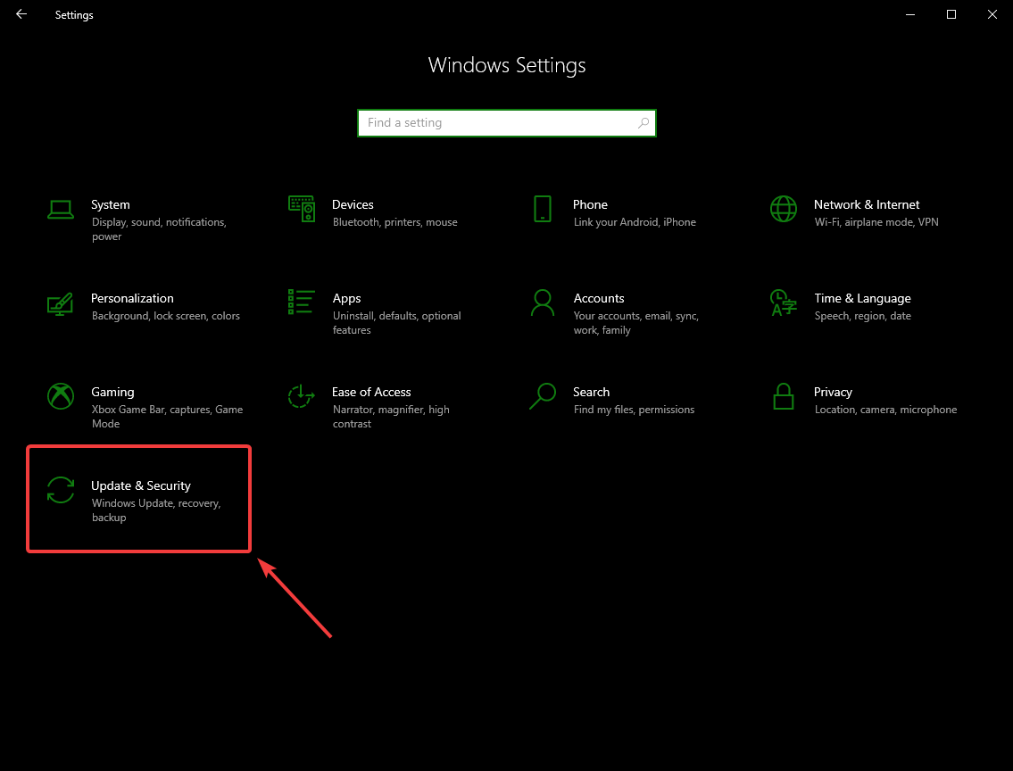
In the right pane, select Open Windows Security
In the left pane, select Firewall and network protection
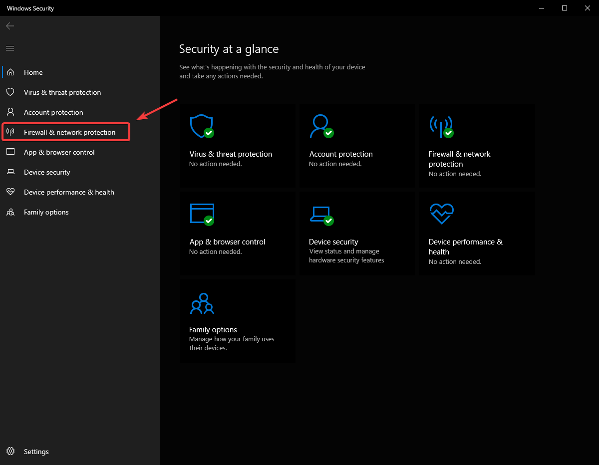
Click on each of the highlighted options
Then click on the On toggle to turn it off.
Click Start -> Control Panel to open the Control Panel. Click the dropdown next to View by: and select Small icons then click Windows Firewall.
In the left pane, click Turn Windows Defender Firewall on or off, and click yes. Enter your Administrator password if a dialog appears.
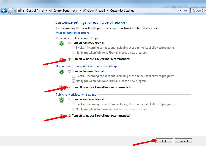
For each category, select the radio button to Turn off Windows Defender Firewall. Then click OK.
Whitelisting Apps
Alternatively, you can add exceptions to the Firewall for any FRC programs you are having issues with.
Click Start -> Settings
Click Update & Security
In the right pane, select Open Windows Security
In the left pane, select Firewall and network protection
At the bottom of the window, select Allow an app through firewall
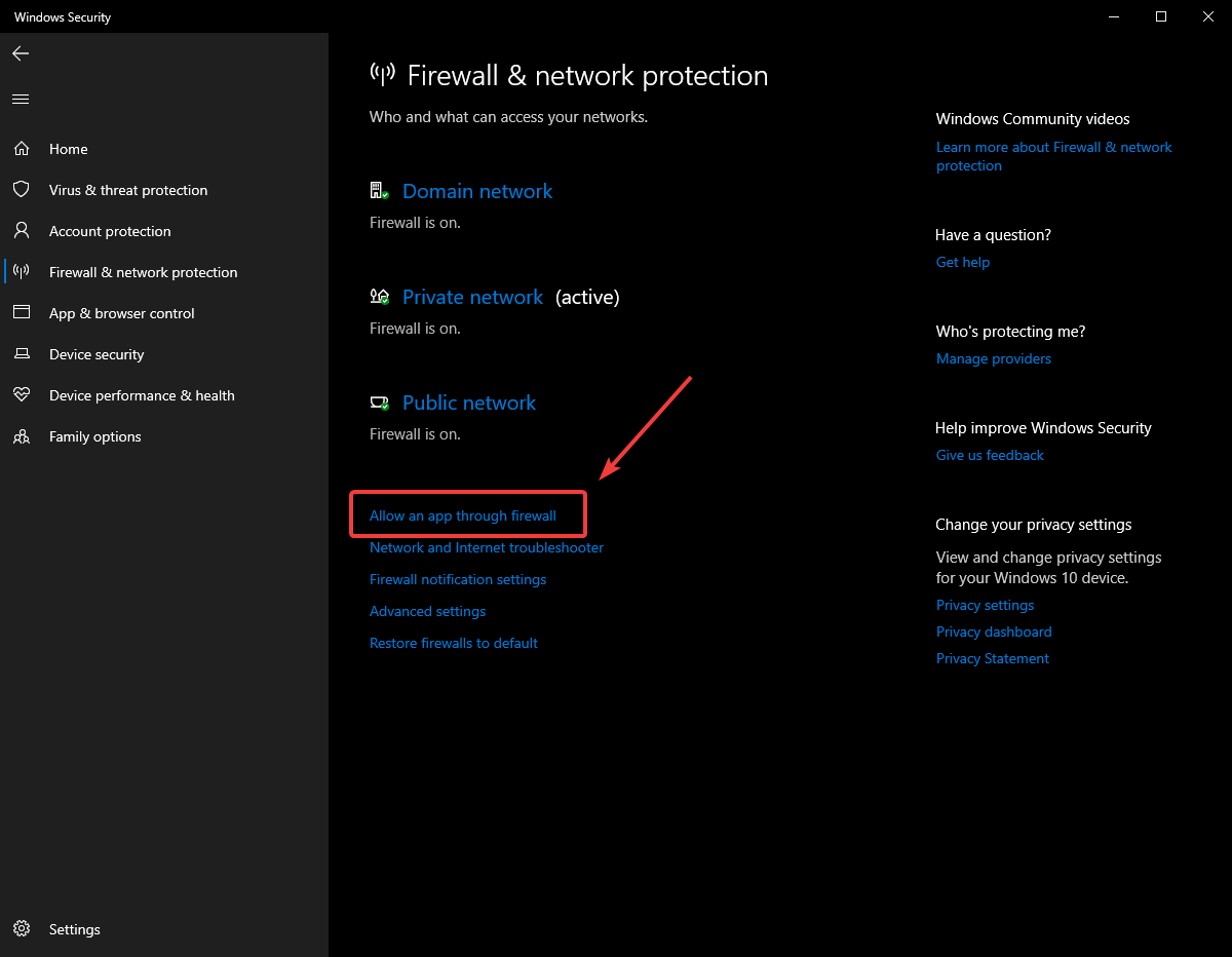
For each FRC program you are having an issue with, make sure that it appears in the list and that it has a check in each of the 3 columns. If you need to change a setting, you made need to click the Change settings button in the top right before changing the settings. If the program is not in the list at all, click the Allow another program… button and browse to the location of the program to add it.
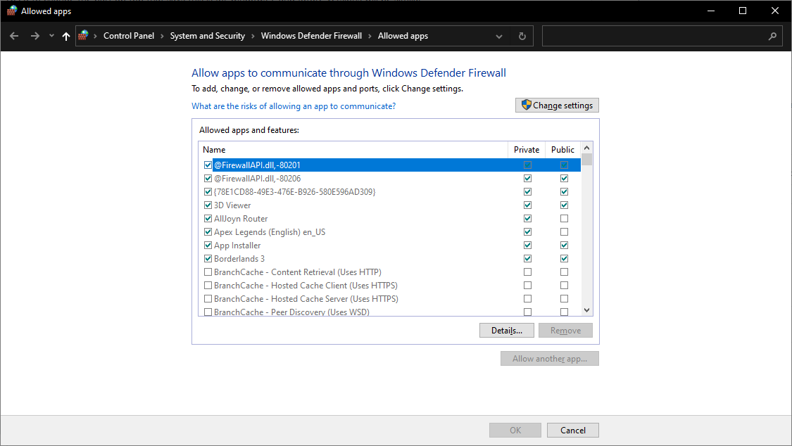
Click Start -> Control Panel to open the Control Panel. Click the dropdown next to View by: and select Small icons then click Windows Defender Firewall.
In the left pane, click Allow a program or feature through Windows Defender Firewall
For each FRC program you are having an issue with, make sure that it appears in the list and that it has a check in each of the 3 columns. If you need to change a setting, you made need to click the Change settings button in the top right before changing the settings. If the program is not in the list at all, click the Allow another program… button and browse to the location of the program to add it.
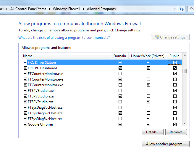
Measuring Bandwidth Usage
On the FRC® Field each team is allocated limited network bandwidth (see R704 in the 2022 manual). The FMS Whitepaper provides more information on determining the bandwidth usage of the Axis camera, but some teams may wish to measure their overall bandwidth consumption. This document details how to make that measurement.
Note
Teams can simulate the bandwidth throttling at home using the FRC Bridge Configuration Utility with the bandwidth checkbox checked.
Measuring Bandwidth Using the Performance Monitor (Win 7 only)
Windows contains a built-in tool called the Performance Monitor that can be used to monitor the bandwidth usage over a network interface.
Launching the Performance Monitor
Click Start and in the search box, type perfmon.msc and press Enter.
Open Real-Time Monitor
In the left pane, click Performance Monitor to display the real-time monitor.
Add Network Counter
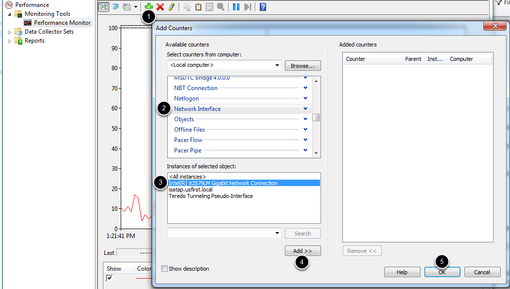
Click the green plus near the top of the screen to add a counter
In the top left pane, locate and click on
Network Interfaceto select itIn the bottom left pane, locate the desired network interface (or use All instances to monitor all interfaces)
Click
Add>>to add the counter to the right pane.Click
OKto add the counters to the graph.
Remove Extra Counters
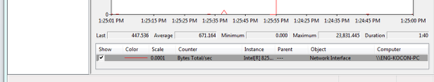
In the bottom pane, select each counter other than Bytes Total/sec and press the Delete key. The Bytes Total/sec entry should be the only entry remaining in the pane.
Configure Data Properties
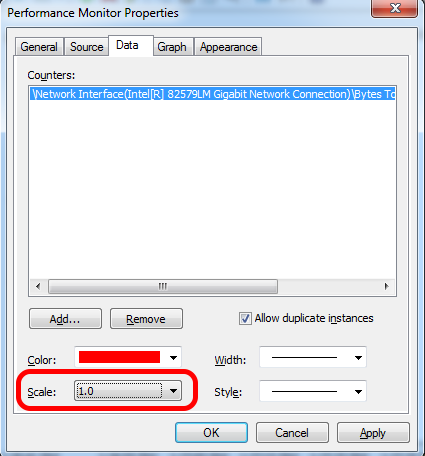
Press Ctrl+Q to bring up the Properties window. Click on the dropdown next to Scale and select 1.0. Then click on the Graph tab.
Configure Graph Properties
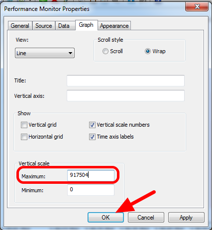
In the Maximum Box under Vertical Scale enter 917504 (this is 7 Megabits converted to Bytes). If desired, turn on the horizontal grid by checking the box. Then click OK to close the dialog.
Viewing Bandwidth Usage
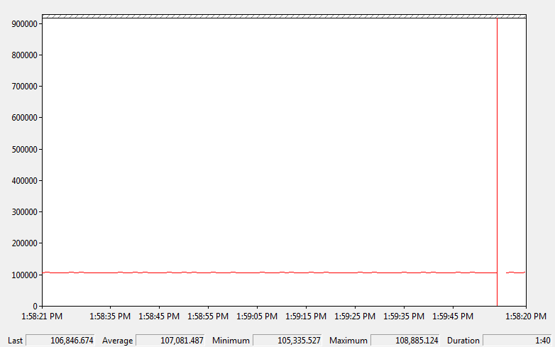
You may now connect to your robot as normal over the selected interface (if you haven’t done so already). The graph will show the total bandwidth usage of the connection, with the bandwidth cap at the top of the graph. The Last, Average, Min and Max values are also displayed at the bottom of the graph. Note that these values are in Bytes/Second meaning the cap is 917,504. With just the Driver Station open you should see a flat line at ~100000 Bytes/Second.
Measuring Bandwidth Usage using Wireshark
If you are not using Windows 7, you will need to install a 3rd party program to monitor bandwidth usage. One program that can be used for this purpose is Wireshark. Download and install the latest version of Wireshark for your version of Windows. After installation is complete, locate and open Wireshark. Connect your computer to your robot, open the Driver Station and any Dashboard or custom programs you may be using.
Select the interface and Start capture
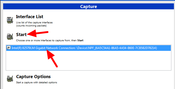
In the Wireshark program on the left side, select the interface you are using to connect to the robot and click Start.
Open Statistics Summary
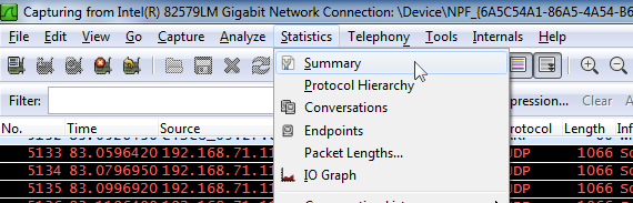
Let the capture run for at least 1 minute, then click Statistics then Summary.
View Bandwidth Usage
Average bandwidth usage, in Megabits/Second is displayed near the bottom of the summary window.
OM5P-AC Radio Modification
The intended use case for the OM5P-AC radio does not subject it to the same shocks and forces as it sees in the FRC® environment. If the radio is subjected to significant pressure on the bottom of the case, it is possible to cause a radio reboot by shorting a metal shield at the bottom of the radio to some exposed metal leads on the bottom of the board. This article details a modification to the radio to prevent this scenario.
Warning
It takes significant pressure applied to the bottom of the case to cause a reboot in this manner. Most FRC radio reboot issues can be traced to the power path in some form. We recommend mitigating this risk via strategic mounting of the radio rather than opening and modifying the radio (and risk damaging delicate internal components):
Avoid using the “mounting tab” features on the bottom of the radio.
You may wish to mount the radio to allow for some shock absorption. A little can go a long way, mounting the radio using hook and loop fastener or to a robot surface with a small amount of flex (plastic or sheet metal sheet, etc.) can significantly reduce the forces experienced by the radio.
Opening the Radio
Note
The OpenMesh OM5P-AC is not designed to be a user serviceable device. Users perform this modification at their own risk. Make sure to work slowly and carefully to avoid damaging internal components such as radio antenna cables.
Case Screws
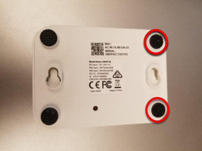
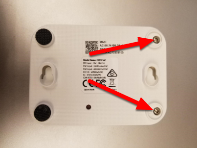
Locate the two rubber feet on the front side of the radio then pry them off the radio using fingernails, small flat screwdriver, etc. Using a small Phillips screwdriver, remove the two screws under the feet.
Side Latches
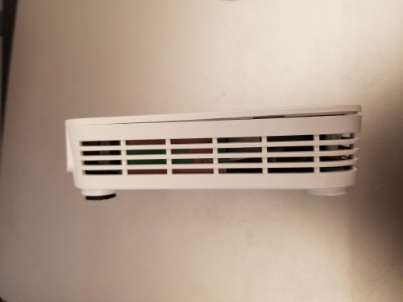
There is a small latch on the lid of the radio near the middle of each long edge (you can see these latches more clearly in the next picture). Using a fingernail or very thin tool, slide along the gap between the lid and case from front to back towards the middle of the radio, you should hear a small pop as you near the middle of radio. Repeat on the other side (note: it’s not hard to accidentally re-latch the first side while doing this, make sure both sides are unlatched before proceeding). The radio lid should now be slightly open on the front side as shown in the image above.
Remove Lid
Warning
The board may stick to the lid as you remove it due to the heatsink pads. Look through the vents of the radio as you remove the lid to see if the board is coming with it, if it is you may need to insert a small tool to hold the board down to separate it from the lid. We recommend a small screwdriver or similar tool that fits through the vents, applied through the front corner on the barrel jack side, right above the screw hole. You can scroll down to the picture with the lid removed to see what the board looks like in this area.
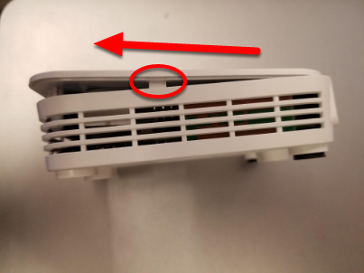
To begin removing the lid, slide it forward (lifting slightly) until the screw holders hit the case front (you may need to apply pressure on the latch areas while doing this.

Next, begin rotating the lid slightly away from the barrel jack side, as shown while continuing to lift. This will unhook the lid from the small triangle visible in the top right corner. Continue to rotate slightly in this direction while pushing the top left corner towards the barrel jack (don’t try to lift further in this step) to unhook a similar feature in the top left corner. Then lift the lid completely away from the body.
Remove Board
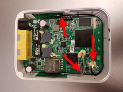
Warning
Note the antenna wires shown in the image above. These wires, and their connectors, are fragile, take care not to damage them while performing the next steps.
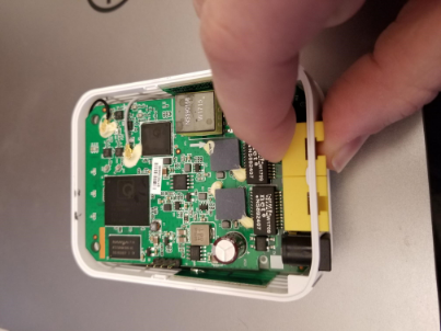
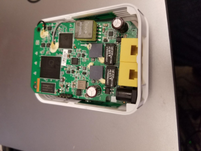
To remove the board, we recommend grasping one or both network ports with your fingers (as shown) and pushing inward (toward the front of the radio) and upward until the network ports and barrel jack are free from the case.
Tilt the board up (towards the short grey antenna cable) to expose the metal shield underneath.
Note
When you perform this step, you may notice that there is a small reset button on the underside of the board that is larger than the hole in the case. Note that pressing the reset button with the FRC firmware installed has no effect and that drilling the case of the radio is not a permitted modification.
Apply Tape
Apply a piece of electrical tape to the metal shield in the area just inside of the network port/barrel jack openings. This will prevent the exposed leads on the underside of the board from short circuiting on this plate.
Re-assemble Radio
Re-assemble the radio by reversing the instructions to open it:
Lay the board back down, making sure it aligns with the screw holes near the front and seats securely
Slide the lid onto the back left retaining feature by moving it in from right to left. Take care of the capacitor in this area
Rotate the lid, press downwards and slide the back right retaining feature in
Press down firmly on the front/middle of the lid to seat the latches
Replace 2 screws in front feet
Replace front feet
Networking Utilities
Port Forwarding
This class provides an easy way to forward local ports to another host/port. This is useful to provide a way to access Ethernet-connected devices from a computer tethered to the roboRIO USB port. This class acts as a raw TCP port forwarder, this means you can forward connections such as SSH.
Forwarding a Remote Port
Often teams may wish to connect directly to the roboRIO for controlling their robot. The PortForwarding class (Java, C++) can be used to forward the Raspberry Pi connection for usage during these times. The PortForwarding class establishes a bridge between the remote and the client. To forward a port in Java, simply do PortForwarder.add(int port, String remoteName, int remotePort).
@Override
public void robotInit() {
PortForwarder.add(8888, "wpilibpi.local", 80);
}
void Robot::RobotInit {
wpi::PortForwarder::GetInstance().Add(8888, "wpilibpi.local", 80);
}
Important
You can not use a port less than 1024 as your local forwarded port. It is also important to note that you can not use full URLs (http://wpilibpi.local) and should only use IP Addresses or DNS names.
Removing a Forwarded Port
To stop forwarding on a specified port, simply call remove(int port) with port being the port number. If you call remove() on a port that is not being forwarded, nothing will happen.
@Override
public void robotInit() {
PortForwarder.remove(8888);
}
void Robot::RobotInit {
wpi::PortForwarder::GetInstance().Remove(8888);
}
Contributing to frc-docs
Contribution Guidelines
Welcome to the contribution guidelines for the frc®-docs project. If you are unfamiliar to writing in the reStructuredText format, please read up on it here.
Important
FIRST® retains all rights to documentation and images provided. Credit for articles/updates will be in the GitHub commit history.
Mission Statement
The WPILib Mission is to enable FIRST Robotics teams to focus on writing game-specific software rather than focusing on hardware details - “raise the floor, don’t lower the ceiling”. We work to enable teams with limited programming knowledge and/or mentor experience to be as successful as possible, while not hampering the abilities of teams with more advanced programming capabilities. We support Kit of Parts control system components directly in the library. We also strive to keep parity between major features of each language (Java, C++, and NI’s LabVIEW), so that teams aren’t at a disadvantage for choosing a specific programming language.
These docs serve to provide a learning ground for all FIRST Robotics Competition teams. Contributions to the project must follow these core principles.
Community-led documentation. Documentation sources are hosted publicly and the community are able to make contributions
Structured, well-formatted, clean documentation. Documentation should be clean and easy to read, from both a source and release standpoint
Relevant. Documentation should be focused on the FIRST Robotics Competition.
Please see the Style Guide for information on styling your documentation.
Release Process
frc-docs uses a special release process for handling the main site /stable/ and the development site /latest/. This flow is detailed below.
During Season:
Commit made to
mainbranchUpdates
/stable/and/latest/on the website
End of Season:
Repository is tagged with year, for archival purposes
Off-Season:
stablebranch is locked to the last on-season commitCommit made to
mainbranchOnly updates
/latest/on the documentation site
Creating a PR
PRs should be made to the frc-docs repo on GitHub. They should point to the main branch and not stable.
Creating New Content
Thanks for contributing to the frc-docs project! There are a couple things you should know before getting started!
Where to place articles?
The location for new articles can be a pretty opinionated subject. Standalone articles that fall well into an already subject category should be placed into mentioned subject category (documentation on something about simulation should be placed into the simulation section). However, things can get pretty complicated when an article combines or references two separate existing sections. In this situation, we advise the author to open an issue on the repository to get discussion going before opening the PR.
Note
All new articles will undergo a review process before being merged into the repository. This review process will be done by members of the WPILib team. New Articles must be on official FIRST supported Software and Hardware. Documentation on unofficial libraries or sensors will not be accepted. This process may take some time to review, please be patient.
Where to place sections?
Sections are quite tricky, as they contain a large amount of content. We advise the author to open an issue to gather discussion before opening up a PR.
Linking Other Articles
In the instance that the article references content that is described in another article, the author should make best effort to link to that article upon the first reference.
Imagine we have the following content in a drivetrain tutorial:
Teams may often need to test their robot code outside of a competition. :ref:`Simulation <link-to-simulation:simulation>` is a means to achieve this. Simulation offers teams a way to unit test and test their robot code without ever needing a robot.
Notice how only the first instance of Simulation is linked. This is the structure the author should follow. There are times where a linked article has different topics of content. If you reference the different types of content in the article, you should link to each new reference once (except in situations where the author has deemed it appropriate otherwise).
Style Guide
This document contains the various RST/Sphinx specific guidelines for the frc-docs project. For guidelines related to the various WPILib code projects, see the WPILib GitHub
Filenames
Use only lowercase alphanumeric characters and - (minus) symbol.
For documents that will have an identical software/hardware name, append “Hardware” or “Software” to the end of the document name. IE, ultrasonics-hardware.rst
Suffix filenames with the .rst extension.
Note
If you are having issues editing files with the .rst extension, the recommended text editor is Notepad++. Please make sure that tabs are replaced with spaces, and the space indentation is set to 3.
Page References
Pages references will be auto-generated based on the page filename and section title.
For example, given the following file contributing.rst and a section called Page References, you would reference this by doing :ref:`contributing:Page References`
Note
Please note that document structure is preserved in references, with the root being the location of the conf.py file. To access documents in sub-folders, simply prepend the folder path before the filename. IE, :ref:`docs/software/hardware-apis/sensors/ultrasonics-sensors:Ultrasonics - Sensors`
Text
All text content should be on the same line, if you need readability, use the word-wrap function of your editor.
Use the following case for these terms:
roboRIO (not RoboRIO, roboRio, or RoboRio)
LabVIEW (not labview or LabView)
Visual Studio Code (VS Code) (not vscode, VScode, vs code, etc)
macOS (not Mac OS, Mac OSX, Mac OS X, Mac, Mac OS, etc.)
GitHub (not github, Github, etc)
PowerShell (not powershell, Powershell, etc)
Linux (not linux)
Java (not java)
Use the ASCII character set for English text. For special characters (e.g. Greek symbols) use the standard character entity sets.
Use .. math:: for standalone equations and :math: for inline equations. A useful LaTeX equation cheat sheet can be found here.
Use literals for filenames, function, and variable names.
Use of the registered trademarks FIRST® and FRC® should follow the Policy from this page. Specifically, where possible (i.e. not nested inside other markup or in a document title), the first use of the trademarks should have the ® symbol and all instances of FIRST should be italicized. The ® symbol can be added by using .. include:: <isonum.txt> at the top of the document and then using *FIRST*\ |reg| or FRC\ |reg|.
Commonly used terms should be added to the FRC Glossary. You can reference items in the glossary by using :term:`deprecated`.
Whitespace
Indentation
Indentation should always match the previous level of indentation unless you are creating a new content block.
Indentation of content directives as new line .. toctree:: should be 3 spaces.
Blank Lines
There should be 1 blank lines separating basic text blocks and section titles. There should be 1 blank line separating text blocks and content directives.
Interior Whitespace
Use one space between sentences.
Headings
Headings should be in the following structure. Heading underlines should match the same number of characters as the heading itself.
=for document titles. Do not use this more than once per article.-for document sections^for document sub-sections~for document sub-sub-sectionsIf you need to use any lower levels of structure, you’re doing things wrong.
Use title case for headings.
Lists
Lists should have a new line in between each indent level. The highest indent should have 0 indentation, and subsequent sublists should have an indentation starting at the first character of the previous indentation.
- Block one
- Block two
- Block three
- Sub 1
- Sub 2
- Block four
Code blocks
All code blocks should have a language specified.
Exception: Content where formatting must be preserved and has no language. Instead use
text.
Follow the WPILib style guide for C++ and Java example code. For example, use two spaces for indentation in C++ and Java.
RLI (Remote Literal Include)
When possible, instead of using code blocks, an RLI should be used. This pulls code lines directly from GitHub, most commonly using the example programs. This automatically keeps the code up to date with any changes that are made. The format of an RLI is:
.. group-tab:: Java
.. rli:: https://raw.githubusercontent.com/wpilibsuite/allwpilib/v2022.2.1/wpilibjExamples/src/main/java/edu/wpi/first/wpilibj/examples/ramsetecontroller/Robot.java
:language: java
:lines: 44-61
:linenos:
:lineno-start: 44
.. group-tab:: C++
.. rli:: https://raw.githubusercontent.com/wpilibsuite/allwpilib/v2022.2.1/wpilibcExamples/src/main/cpp/examples/RamseteController/cpp/Robot.cpp
:language: cpp
:lines: 18-30
:linenos:
:lineno-start: 18
Note that group-tab rather than code-tab needs to be used. Also make sure to link to the raw version of the file on GitHub, there is a handy Raw button in the top right corner of the page.
Admonitions
Admonitions (list here) should have their text on the same line as the admonition itself. There are exceptions to this rule however, when having multiple sections of content inside of admonition. Generally having multiple sections of content inside of an admonition is not recommended.
Use
.. warning:: This is a warning!
NOT
.. warning::
This is a warning!
Links
It is preferred to format links as anonymous hyperlinks. The important thing to note is the two underscores appending the text. In the situation that only one underscore is used, issues may arise when compiling the document.
Hi there, `this is a link <https://example.com>`__ and it's pretty cool!
However, in some cases where the same link must be referenced multiple times, the syntax below is accepted.
Hi there, `this is a link`_ and it's pretty cool!
.. _this is a link: https://example.com
Images
Images should be created with 1 new line separating content and directive.
All images (including vectors) should be less than 500 kilobytes in size. Please make use of a smaller resolution and more efficient compression algorithms.
.. image:: images/my-article/my-image.png
:alt: Always add alt text here describing the image.
Image Files
Image files should be stored in the document directory, sub-directory of document-name/images
They should follow the naming scheme of short-description.png, where the name of the image is a short description of what the image shows. This should be less than 24 characters.
They should be of the .png or .jpg image extension. .gif is unacceptable due to storage and accessibility concerns.
Note
Accessibility is important! Images should be marked with a :alt: directive.
.. image:: images/my-document/my-image.png
:alt: An example image
Vector Images
SVG files are supported through the svg2pdfconverter Sphinx extension.
Simply use them as you would with any other image.
Note
Ensure that any embedded images in the vector do not bloat the vector to exceed the 500KB limit.
.. image:: images/my-document/my-image.svg
:alt: Always add alt text here describing the image.
Draw.io Diagrams
Draw.io (also known as diagrams.net) diagrams are supported through svg files with embedded .drawio metadata, allowing the svg file to act as a source file of the diagrams, and to be rendered like a normal vector graphics file.
Simply use them like you would any other vector image, or any other image.
.. image:: diagrams/my-document/diagram-1.drawio.svg
:alt: Always add alt text here describing the image.
Draw.io Files
Draw.io files follow almost the same naming scheme as normal images. To keep track of files that have the embedded .drawio metadata, append a .drawio to the end of the file name, before the extension, meaning the name of the file should be document-title-1.drawio.svg and so on. Additionally, diagrams should be stored in the document directory in a sub-folder named diagrams.
For the specifics of saving a diagram as a .svg with metadata, take a look at Draw.io Saving Instructions.
Warning
Make sure you don’t modify any file that is in a diagrams folder, or ends in .drawio.svg in any program other than draw.io, otherwise you might risk breaking the metadata of the file, making it uneditable.
File Extensions
File extensions should use code formatting. For example, use:
``.png``
instead of:
.png
".png"
"``.png``"
Table of Contents (TOC)
Each category should contain an index.rst. This index file should contain a maxdepth of 1. Sub-categories are acceptable, with a maxdepth of 1.
The category index.rst file can then be added added to the root index file located at source/index.rst.
Examples
Title
=====
This is an example article
.. code-block:: java
System.out.println("Hello World");
Section
-------
This is a section!
Important Note!
This list is not exhaustive and administrators reserve the right to make changes. Changes will be reflected in this document.
Build Instructions
This document contains information on how to build the HTML, PDF, and EPUB versions of the frc-docs site. frc-docs uses Sphinx as the documentation generator. This document also assumes you have basic knowledge of Git and console commands.
Prerequisites
Ensure that Git is installed and that the frc-docs repository is cloned by using git clone https://github.com/wpilibsuite/frc-docs.git.
Windows
Note
MikTeX and rsvg-convert are not required for building HTML, they are only required for Windows PDF builds.
Python 3.6 or greater (docs are tested using 3.8)
MiKTeX (Only needed for PDF builds)
Ensure that Python is in your Path by selecting the Add Python to PATH toggle when installing Python.
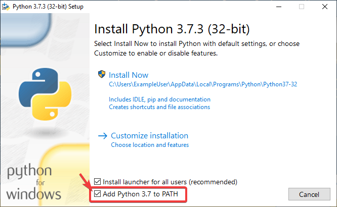
Once Python is installed, open up Powershell. Then navigate to the frc-docs directory. Run the following command: pip install -r source/requirements.txt
Install the missing MikTex packages by navigating to the frc-docs directory, then running the following command from Powershell: mpm --verbose --require=@miktex-packages.txt
Linux (Ubuntu)
$ sudo apt update
$ sudo apt install python3 python3-pip
$ python3 -m pip install -U pip setuptools wheel
$ python3 -m pip install -r source/requirements.txt
$ sudo apt install -y texlive-latex-recommended texlive-fonts-recommended texlive-latex-extra latexmk texlive-lang-greek texlive-luatex texlive-xetex texlive-fonts-extra dvipng librsvg2-bin
Building
Open up a Powershell Window or terminal and navigate to the frc-docs directory that was cloned.
PS > cd "%USERPROFILE%\Documents"
PS C:\Users\Example\Documents> git clone https://github.com/wpilibsuite/frc-docs.git
Cloning into 'frc-docs'...
remote: Enumerating objects: 217, done.
remote: Counting objects: 100% (217/217), done.
remote: Compressing objects: 100% (196/196), done.
remote: Total 2587 (delta 50), reused 68 (delta 21), pack-reused 2370
Receiving objects: 100% (2587/2587), 42.68MiB | 20.32 MiB/s, done.
Receiving deltas: 100% (1138/1138), done/
PS C:\Users\Example\Documents> cd frc-docs
PS C:\Users\Example\Documents\frc-docs>
Lint Check
Note
Lint Check will not check line endings on Windows due to a bug with line endings. See this issue for more information.
It’s encouraged to check any changes you make with the linter. This will fail the buildbot if it does not pass. To check, run .\make lint
Link Check
The link checker makes sure that all links in the documentation resolve. This will fail the buildbot if it does not pass. To check, run .\make linkcheck
Image Size Check
Please run .\make sizecheck to verify that all images are below 500KB. This check will fail CI if it fails. Exclusions are allowed on a case by case basis and are added to the IMAGE_SIZE_EXCLUSIONS list in the configuration file.
Redirect Check
Files that have been moved or renamed must have their new location (or replaced with 404) in the redirects.txt file in source.
The redirect writer will automatically add renamed/moved files to the redirects file. Run .\make rediraffewritediff.
Note
if a file is both moved and substantially changed, the redirect writer will not add it to the redirects.txt file, and the redirects.txt file will need to be manually updated.
The redirect checker makes sure that there are valid redirects for all files. This will fail the buildbot if it does not pass. To check, run .\make rediraffecheckdiff to verify all files are redirected. Additionally, an HTML build may need to be ran to ensure that all files redirect properly.
Building HTML
Type the command .\make html to generate HTML content. The content is located in the build/html directory at the root of the repository.
Building PDF
Warning
Please note that PDF build on Windows may result in distorted images for SVG content. This is due to a lack of librsvg2-bin support on Windows.
Type the command .\make latexpdf to generate PDF content. The PDF is located in the build/latex directory at the root of the repository.
Building EPUB
Type the command .\make epub to generate EPUB content. The EPUB is located in the build/epub directory at the root of the repository.
Adding Python Third-Party libraries
Important
After modifying frc-docs dependencies in any way, requirements.txt must be regenerated by running poetry export -f requirements.txt --output source/requirements.txt --without-hashes from the root of the repo.
frc-docs uses Poetry to manage its dependencies to make sure builds are reproducible.
Note
Poetry is not required to build and contribute to frc-docs content. It is only used for dependency management.
Installing Poetry
Ensure that Poetry is installed. Run the following command: pip install poetry
Adding a Dependency
Add the dependency to the [tool.poetry.dependencies] section of pyproject.toml. Make sure to specify an exact version. Then, run the following command: poetry lock --no-update
Updating a Top-Level Dependency
Update the dependency’s version in the [tool.poetry.dependencies] section of pyproject.toml. Then, run the following command: poetry lock --no-update
Draw.io Saving Instructions
Warning
Make sure you don’t modify any file that is in a diagrams folder, or ends in .drawio.svg in any program other than draw.io, otherwise you might risk breaking the metadata of the file, making it uneditable.
Draw.io (also known as diagrams.net) are supported when saved as svg files, with embedded XML metadata for the draw.io source file (normally stored as .drawio).
This allows these images to both act as source files for the diagrams that can be edited in the future, and be rendered as normal svg files.
There are a few methods to save a diagram with the embedded metadata, but using the export menu is preferred because it allows us to embed any images in the diagram, otherwise they might not render properly on the docs.
This method is applicable to both draw.io desktop and the web version at diagrams.net.
To export go to File - Export as - SVG.... Make sure Include a copy of my diagram is enabled to embed the diagram metadata, and that Embed Images is enabled so image files in the diagram are embedded so they render in the docs. Additionally, mark the Transparent Background option to make sure the background is displayed correctly.
The export menu should look something like this:
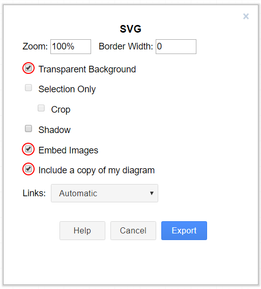
Then just click Export then select where you would like to save the file and save it.
Note
When saving, make sure you follow the style-guide at Draw.io Files
Translations
frc-docs supports translations using the web-based Transifex utility. frc-docs has been translated into Spanish - Mexico (es_MX), French - Canada (fr_CA) and Turkish - Turkey (tr_TR). Chinese - China (zh_CN), Hebrew - Israel (he_IL), and Portuguese - Brazil (pt_BR) have translations in progress. Translators that are fluent in both English and one of the specified languages would be greatly appreciated to contribute to the translations. Even once a translation is complete, it needs to be updated to keep up with changes in frc-docs.
Workflow
Here are some steps to follow for translating frc-docs.
Sign up for Transifex and ask to join the frc-docs project, and request access to the language you’d like to contribute to.
Join GitHub discussions! This is a direct means of communication with the WPILib team. You can use this to ask us questions in a fast and streamlined fashion.
You may be contacted and asked questions involving contributing languages before being granted access to the frc-docs translation project.
Translate your language!
Links
Links must be preserved in their original syntax. To translate a link, you can replace the TRANSLATE ME text (this will be replaced with the English title) with the appropriate translation.
An example of the original text may be
For complete wiring instructions/diagrams, please see the :doc:`Wiring the FRC Control System Document <Wiring the FRC Control System document>`.
where the Wiring the FRC Control System Document then gets translated.
For complete wiring instructions/diagrams, please see the :doc:`TRANSLATED TEXT <Wiring the FRC Control System document>`.
Another example is below
For complete wiring instructions/diagrams, please see the :ref:`TRANSLATED TEXT <docs/zero-to-robot/step-1/how-to-wire-a-robot:How to Wire an FRC Robot>`
Publishing Translations
Translations are pulled from Transifex and published automatically each day.
Top Contributors
Daltz333 - 295 contributions
sciencewhiz - 235 contributions
Oblarg - 107 contributions
prateekma - 84 contributions
jasondaming - 77 contributions
benjamin-antupit - 46 contributions
AustinShalit - 44 contributions
Kevin-OConnor - 32 contributions
TheTripleV - 27 contributions
Starlight220 - 23 contributions
Top Translators
Chinese
8192 Dhc
Atlus Zhang
Jiangshan Gong
Keseterg
Michael Zhao
Ningxi Huang
Ran Xin
Team 5308
Tianrui Wu
Tianshuang Zhang
Xun Sun
Yitong Zhao
Yuhao Li
堂晋 徐
志鹏 邢
怡静 陆
智翔 杨
楚涵 张
璨宇 汤
陈 Sherry
French
Alexandra Schneider
Andre Theberge
Andy Chang
Austin Shalit
Dalton Smith
Daniel Renaud
Étienne Beaulac
Félix Giffard
Kaitlyn Kenwell
Laura Luna Bedard
Martin Regimbald
Regis Bekale
Sami G.-D.
Youdlain Marcellus
Portuguese
Amanda Carolina Wilmsen
Bibiana Oliveira
Bruno Osio
Bruno Toso
Gabriel Silveira
Gabriela Tomaz Do Amaral Ribeiro
Günther Steinmeier
Karana Maciel De Souza
Luca Carvalho
Lucas Fontes Francisco
Matheus Heitor Timm Chanan
Meg Grabin
Nadja Dias
Natan Feijó Tristão
Nathany Santiago
Pedro Henrique Dias Pellicioli
Tales Dias De Almeida Silva
Vinícius Castro
Spanish
Austin Shalit
Daniel Núñez
Diana Ramos
Emiliano Vargas
Fernanda Reveles
Fernando Soltero
Gibrán Verástegui
Heber Sepúlveda
Heriberto Gutierrez
Hugo Espino
Karina Torres
Lian Eng
Luis_Hernández
Miguel Angel De León Adame
Paulina Maynez
Pierre Cote
Ranferi Lozano
Rodrigo Acosta
Sofia Fernandez
Zara Moreno
Turkish
Hasan Bilgin
Müfit Alkaya
Esra Özemre
Demet T
Ceren Oktemer
Demet Tumkaya
Melis Aldeniz
Duru Ünlü
Arhan Ünay
Müfit Alkaya_3390
Nesrin Serra Köşkeroğlu
Duru Hatipoğlu
Ada Zagyapan
Mufit Alkaya
Kaan Çakıl
Yaren K
Ege Feyzioglu
Eray Özsaray
Seda Kılıçaslan
Deniz Ornek
Hebrew
Aric Radzin
Dalton Smith
Itay Ziv
Ofek Ashery
Starlight220
Yotam Shlomi